Technical Terms
Please click on the red arrows to open the text under each subject heading.
Efficiency and Losses
Thermal Efficiency
The “thermal efficiency” of any engine is defined as the amount of useful energy output divided by the amount of energy input . It is not a fixed quantum but varies according to the engine’s load and conditions of operation.
In the case of steam locomotives, the term thermal efficiency may refer to “Cylinder or Indicated Efficiency“, “Drawbar Thermal Efficiency” or even “Boiler Efficiency“. These are described on separate pages, however their definitions are importantly different as outlined below: Three types of efficiency are described on separate pages as follows:
- Cylinder efficiency is defined as the the amount of energy delivered by the cylinder to the piston divided by the amount of energy delivered to the cylinder in the form of steam delivered to the steamchest;
- Drawbar efficiency is defined as the the amount of energy delivered at the locomotive’s drawbar (the hook at the back of its tender) divided by the amount of energy available in the fuel placed into its firebox.
- Boiler efficiency can be defined as the amount of energy delivered from the boiler in the form of steam divided by the amount of energy delivered to the firebox in the form of fuel/chemical energy.
Both the cylinder and drawbar efficiencies vary with speed and power output, maximum cylinder efficiency being achieved at much higher speed than maximum drawbar efficiency. This is because, as speed rises, a locomotive’s rolling resistance also rises and the tractive force avalable at its drawbar falls until, at a certain speed, the drawbar force becomes zero and thus the drawbar efficiency also becomes zero.
Cylinder efficiency is calculated by dividing the work done by the steam in the cylinder by the heat drop in the cylinder.
In Line 84 of FDC 1.3, Wardale calculates the isentropic cylinder efficiency of the 5AT at maximum drawbar power output to be 81%. He gets this figure by dividing the actual specific work done by the cylinder in kJ/kg (calculated from the indicator diagram) by the isentropic heat drop in the cylinder (also in kJ/kg) measured from an h-s chart (click on link to see chart and explanation).
Cylinder efficiency is governed by the shape of the Indicator Diagram and in particular by the losses that are evidenced by it – most especially expansion losses, condensation losses and leakage losses.
Note: in Line 80 of FDC 1.3, Wardale estimated that the steam flow to the 5AT’s cylinders needed to be increased by 5% above theoretical requirement to allow for “heat transfer to the cylinder walls during steam admission”. He goes on to point out that this low value results from using “all practical features to reduce it, such as:
- very high superheat,
- long stroke:diameter ratio,
- optimum cylinder insulation,
- high rotational speed at normal train speed,
- low clearance volume,
- special engine component design, etc.”
All of these features serve to increase cylinder efficiency.
Limit of Cylinder Efficiency: It should be noted that even with no losses, there is an upper limit to cylinder efficiency governed by Carnot’s equation which states that the maximum theoretical efficiency of any heat engine is governed by the temperature difference between its heat source and its heat sink.
Note: Isentropic efficiency is another (but very different) measure of cylinder efficiency. Instead of describing the ratio of work output to work output, it describes the ratio of work output with maximum possible work output based on steam conditions – see Thermodynamics definitions.
Drawbar efficiency can be seen as the sum of the efficiencies of a locomotive’s various components. Wardale provides examples of these in his book “The Red Devil and Other Tales from the Age of Steam” where (in Table 78, page 457) he quotes figures for standard and (proposed) modified Chinese Class QJ locomotives, and where (on page 501) he suggests what might be achieved from the further development to the level of “Third Generation Steam” traction.
The figures from these pages are combined in a single table below, however it is recommended that the qualifying texts from both Table 78 (page 457) and page 501 of Wardale’s book be read in association with them.
| Item | Standard QJ | Modified QJ | Third Generation Steam |
| Boiler combustion efficiency | 78% | 87% | 95% |
| Boiler absorption efficiency | 78.2% | 80% | 90% |
| Auxiliary efficiency factor | 93.1% | 94% | 96% |
| Cylinder efficiency | 16.4% | 19.05% | 22% |
| Transmission efficiency | 89% | 93% | 94% |
| Drawbar efficiency | 94% | 95% | 96% |
| Overall drawbar thermal efficiency = product of all the above |
7.8% | 11.0% | 16.3%* |
Maximum drawbar thermal efficiency is usually reached at modest speed and power outputs such that increasing rolling resistance and increasing fuel carry-over (in the case of coal firing) are offset by increasing cylinder efficiency.
* Note: Wardale’s estimate for TGS drawbar efficiency differs significantly from the figure of 25% that he quotes as being Porta’s estimate for condensing third generation steam locomotives – see Second Generation Steam page of this website. However Wardale makes it clear (on page 501 of his book) that his figure applies to non-condensing locomotives and that “higher efficiency could only be obtained by expanding the steam to sub-atmospheric pressure and low temperature by means of condensing to counter the negative effect on the cycle efficiency of the restricted inlet steam temperature as done in stationary steam plant”.
Boiler efficiency can be defined as the amount of energy delivered from the boiler in the form of steam divided by the amount of energy delivered to the firebox in the form of fuel/chemical energy.
Boiler efficiency depends on the design of the boiler and firebox, the type of fuel, and the draughting system. In the case of coal-fired boilers, boiler efficiency declines linearly with rate of fuel feed, as discussed on the Grate Limit and Boiler Efficiency page.
Wall Effects and Condensation
NOTE
Since the publication of this page in 2017, new information has become available in the form of correspondence from André Chapelon about the testing of his experimental 2-12-0 6-cylinder compound freight engine No. 160A1, which suggests that steam heating of its cylinders with live steam was effective in overcoming wall effects, suggesting that superheating might be unnecessary. A copy of this correspondence (translated into English by Hendrik Kaptein) can be found in Newsletter No 22 issued Aug 2023.
This subject was further discussed in Newsletter No 28 (Oct 2025) and Newsletter No 29, in which convincing counter-arguments by Jamie Keyte, David Pawson and others were presented.
Wall Effects: The term “wall effects” refers to the changes in steam temperature caused by temperature differentials between the steam and the walls of the cylinder, its end covers and the steam passages connecting to it.
When high temperature, high pressure steam enters the cylinder, it comes into contact with the relatively cool walls. The wall surfaces are cooler than the steam partly because they lose heat by conduction and radiation, but more importantly they are cooled by the steam itself as it expands during the release and exhaust phases of the power cycle. Thus it may be deduced the temperature of these surfaces varies around an average that is a little lower than the average steam temperature over the cycle. As a result, not only are these surfaces cooler than the incoming steam and so absorb heat from it, but they are warmer than the outgoing steam and so give up heat to it.
The fact that heat is transferred from the hot steam to the cylinder walls during the expansion phase and heat is transferred to the walls during the beginning of the compression phase, means that both these phases are not adiabatic
In consequence, the expansion index (n in the equation PVn = k) during these phases varies from a maximum (adiabatic) value of 1.3 to maybe 1.2 or in the case of short cut-off working and slow rotational speeds, even as low as 1.1.
Note: in Line 80 of FDC 1.3, Wardale estimated that the steam flow to the 5AT’s cylinders should be increased by 5% to allow for “heat transfer to the cylinder walls during steam admission”. He goes on to explain that this low value results from using “all practical features to reduce it, such as very high superheat, long stroke : diameter ratio, optimum cylinder insulation, high rotational speed at normal train speed, low clearance volume, special engine component design, etc.”
Condensation: Because steam locomotives have traditionally been inadequately superheated, the term “wall effects” is often used synomymously with “condensation”.
Condensation of steam inside the cylinder results in a massive waste of energy as described in detail in Porta’s “compounding” paper published in Camden’s book “Advanced Steam Locomotive Development – Three Technical Papers“.
Porta describes wall effects as follows:
“Wall effect phenomena occur as follows. The cylinder cover, the steam passages and the piston (where the wall effects are most intense) are at a temperature between that of the live steam and the exhaust steam. Therefore, when the superheated steam makes contact with them, an energy drop takes place which show as a temperature drop. …. If the temperature of the walls is higher than the saturation temperature, no condensation occurs – the heat transfer being governed by “gas” laws, and is very small. But as shown by experimental data, if the temperature of the confining walls is below the saturation point at steamchest pressure, then condensation occurs even if the steam is highly superheated. This situation is the most frequent one in the life of steam locomotives: one of the causes is poor insulation, leading to heavy cooling down because of the intermittent nature of railway work.
The Author’s measurements, even if rough, show that when the cylinders are well warned up after a lengthy, strenuous pull, in an ordinary locomotive in which the steam temperature attains 400°C, the walls reach a temperature higher than 210°C only at cut-offs greater than ~20%. Therefore, at shorter cut-offs, condensation occurs and the machine works with wall effects approaching those of a saturated one.
The temperature drop (in the case of no condensation, later to be defined) is roughly inversely proportional to the cut-off and to the rotational velocity to the power of -0.3 (ω-0.3). Thus, in the case of shunting locomotives, single expansion engines work with wall effects corresponding to saturated engines working at very low speeds, say ~1 rps, hence very high.
A large number of tests reported by GUTERMUTH show that condensation in saturated engines fed with steam at 8 to 12 bar, between points 6 and 2, Fig. 1, amounts to 40 to 50% of the steam admitted to the cylinder (and even more). And this refers to STATIONARY engines. What can be expected in the case of well “ventilated” [i.e. poorly insulated] locomotive cylinders?”
Fig 1 referred to in the text above is copied below with some corrections. It is also slightly simplified for clarity:
In this diagram, the variable steam inlet pressure between points 1 and 2 is replaced by a straight horizontal line G between 11 to 211 representing the mean pressure of the steam entering the cylinder. The location of this line is derived by equating the hatched areas above and below it.
If steam entering the cylinder comes into contact with surfaces that are below the saturation temperature for the steam, then condensation will occur onto those surfaces. Each cubic centimeter of condensate representing perhaps 1000 cc of useful steam (depending on its pressure). In any case it represents a contraction or loss of steam that is represented by the segment 21 to 211. This in turn results in an irrecoverable* loss of work or energy as represented by the hatched area H.
[* Porta points out that the condensate is likely to vapourize during the compression phase, thus recovering some energy that supplements the draught created by the exhaust system. This is offers no compensation for the loss of energy that might otherwise have been used for moving the locomotive and its train.]
In his “Compounding” paper, Porta goes on to say that:
“the basic principal concerning wall effects is to have at all times the temperature of the walls above the saturation point. It is therefore essential to have the highest possible steam temperature, even beyond the theoretical optimum. This point was missed by Churchward and all the British designers who followed him, with the possible exception of Gresley. The Americans also missed it.
The Author coined the expression “exaggerated insulation” (“hyper-exaggerated” for fireless locomotives) which implies the substitution of sealed-for-life fibreglass type material in place of cancer-causing, and less efficient, asbestos, and also the concept of insulating the whole cylinder front end, including the smokebox saddle, and its bottom, comprising the frame. Perhaps the most important point is that of keeping the cylinders hot between the working spells inherent to the intermittent nature of railway service. The “sealed-for-life” concept is a critical part of this; Wardale reported that in South Africa some 70% of the locomotives had no insulation at all!
A further attack on the problem could be the application of ceramic coatings on the surfaces: around 1890 Thurston (a very clever man) proposed painting these with a mixture of graphite and linseed oil. The Author tried it, but for trivial reasons the experiment was not followed up.
Another means of reducing wall effects to negligible proportions is to use steam jackets, but not those adopted by Chapelon for the 160A1 which required very complex castings. A welded fabrication is much simpler. These should be fitted to the cylinder covers, and around the steam passages, but NOT to the cylinder barrel. Jackets can also be fitted to the cylinders of fireless engines operating with saturated steam. Another difference from Chapelon’s scheme is that the jacket condensation is not mixed up with the main steam flow, but re-injected to the hot water reservoir.
Porta makes the point that condensation is equivalent to steam loss which necessarily increases steam consumption, and that this this directly reduces a locomotive power output as illustrated by his oft-repeated equation:

Porta concludes that wall effects or condensation can be minimised by:
- Using the highest possible superheat temperatures;
- Providing the best possible insulation of all external hot surfaces such as cylinders, cylinder covers, valves, steam chests and even the smokebox saddle to which steamchests and cylinders are connected;
- Providing steam heating to cylinder covers (but not cylinders);
- Using the smallest possible wheel diameter to maintain a high revolution rate;
- Using the smallest possible cylinder diameter and long stroke.
He also points out that:
- Short cut-off working results in lower surface temperatures and increased likelihood of condensation. Better to operate at >20% cut-off, illustrating one of the advantages of “compound” working;
- Condensation is inevitable during warm-up periods – usually around 20 minutes of operation on full power. Shunting locomotives are likely to suffer from large condensation losses.
- Fireless locomotives operating on saturated steam are also likely to insuffer from large condensation losses.
Several pages of this website include text and diagrams copied from Porta’s “compounding” paper, including the pages covering steam leakage, clearance volume, incomplete expansion and triangular losses. More specific references to his theories on compound expansion can be found on the α Coefficient and Compound Expansion pages.
Sincere thanks to Adam Harris of Camden Miniature Steam, publishers of “Advanced Steam Locomotive Development – Three Technical Papers” for allowing the sections of the book to be published on this website.
Triangular Losses in Cylinders
Page Under Development
This page is still “under development”. Please contact Chris Newman at webmaster@advanced-steam.org if you would like to help by contributing text to this or any other page.
The term “triangular losses” is used to describe the rounding of the corners of a locomotive’s indicator diagram caused by the opening and closing of valves, and whose effect is to reduce the area of the diagram and thus the work done by each piston stroke which in turn reduces power output and efficiency. Some of these do not represent losses of energy so much as “losses of potential”.
Triangular losses are perhaps best described in Porta’s “compounding” paper published in Camden’s book “Advanced Steam Locomotive Development – Three Technical Papers” and consist of the rounded corners of a typical Indicator Diagram as compared to an “Ideal” diagram, as shown on Figure 1 of Porta’s paper as shown on the Condensation and Incomplete Expansion pages of this website.
A simplied indicator diagram is shown below to illustrate triangular losses.

Three loss areas are shown:
- Area A occurs during the steam admission phase where throttling occurs due to the narrowing of the admission port as the valve approaches cut-off;
- Area B occurs when the exhaust port opens before the piston reaches the end of its stroke, allowing the escape of steam before it fully expands into the cylinder;
- Area C is the compression (or pre-compression) that occurs when the exhaust valve closes before the piston reaches the end of its stroke.
It might be argued that Areas A and C should not be regarded as “losses” per se. Triangle A primarily represents lost potential by virtue of steam that failed to enter the cylinder because of throttling during valve closure. (An entropy rise results from the throttling process so some energy loss is involved also).
Triangle C also largely represents lost potential since it is apparent that the area inside the diagram would be larger (and therefore more power gained) if the exhaust port were to stay open until the end of the piston stroke. However, since the steam is compressed elastically it returns most of the energy that it absorbs during the reverse stroke, some being lost through an increase in entropy.
Notwithstanding, pre-compression offers two advantages – (a) it cushions the piston’s inertial (deceleration) forces that would otherwise have to be resisted by the connecting rod and crank pin; and (b) it builds up the cylinder pressure prior to admission and thus helps to reduce or eliminate another triangular loss that would otherwise arise at the top corner of the diagram due to a delayed rise of pressure as steam flows into the empty cylinder when the inlet valve opens.
In fact triangular losses are more complex than shown as ‘A’ in the simplified diagram above. Porta draws attention to the triangular losses that actually occur at the start of admission (as the inlet valve opens) and illustrates his point in Fig 8 of his “Compounding” paper as below:

Note: The “net definite pre-admission that Porta refers to can also be referred to as “lead” as defined in the Valves and Valve Gear page of this website. What he is saying here is that the use of lead causes a small triangular loss (shown with horizontal shading). On the other hand, absense of lead (or inadequate lead) results in a much larger triangular loss (shown with vertical shading).
Porta goes on to point out that the admission losses should actually include the area under the “Nominal Steam Pressure” line (indicated in yellow shading below), demonstrating the importance of (a) operating at maximum boiler pressure; (b) the use of large steam pipes, large steam chest and internal streamlining to minimize the pressure drop between boiler and cylinder.

Conclusion:
Triangular losses cannot be eliminated, but they can be minimized by careful design – for instance:
- use of large valves and port openings to reduce steam velocity and consequent flow losses;
- optimizing valve events using computer simulation such as those of Prof Bill Hall and Dr Allan Wallace;
- in the case of piston valves, by the use of long-travel valves that pass over the ports at higher speed, thereby reducing the time that the entry or exit of steam is throttled through a partialy opened port.
- use large steam chests to minimise steamchest pressure drop during admission – ideally steamchest voiume should equal cylinder volume.
Note: “Losses of potential” (as described above) are real losses in the form of wasted capital rather than wasted energy. Minimizing losses in potential increases a locomotive’s performance and therefore its return on capital.
Porta’s paper titled “Fundamentals of the Porta Compounding System for Steam Locomotives” addresses other associated factors that detract from a locomotive’s cylinder efficiency, including condensation/wall effects, steam leakage, clearance volume and incomplete expansion as described elsewhere on this website. More specific references to his theories on compound expansion can be found on the α Coefficient and Compound Expansion pages.
Sincere thanks to Adam Harris of Camden Miniature Steam, publishers of “Advanced Steam Locomotive Development – Three Technical Papers” for allowing the sections of the book to be published on this website.
Incomplete Expansion of Steam in the Cylinder
Page Under Development
This page is still “under development”. Please contact Chris Newman at webmaster@advanced-steam.org if you would like to help by contributing text to this or any other page.
The term “incomplete expansion” is used to describe the curtailment of the expansion of steam inside a locomotive’s cylinder brought about by the opening of the exhaust valve, thus allowing the remaining energy in the steam to be lost to atmosphere. They may also be described as losses caused by insufficient cylinder volume. Either way, the effect is to limit the work done by each piston stroke which in turn inhibits the locomotive’s power output and efficiency.
Incomplete expansion losses are best visualized diagramatically as shown on the indicator diagram below, copied from Porta’s “Compounding” paper as published in Camden’s book “Advanced Steam Locomotive Development – Three Technical Papers“. The incomplete expansion loss is shown as the hatched area ‘K’.

In his “Compounding” paper, Porta goes on to state:
The loss of the single expansion engine is the incomplete expansion. This loss is heavier the higher the boiler pressure is, indicating the benefits of compounding.
Incomplete expansion also increases with longer cut-off (i.e. fatter indicator diagram) which is why short cut-off working is held to be the secret of economical operation. In fact this is not so, since short cut-off working results in greater cooling of the cylinder walls and a consequential increase the likelihood of condensation as explained in the Condensation page of this website. Porta therefore recommends a cut-off of 20 to 25% for single expansion operation as being a compromise between the conflicting aims of minimizing condensation and minimizing incomplete expansion. It further explains why he recommends compound expansion since this allows the use of much longer cut-offs, resuperheating to prevent all possibility of condensation, and expansion losses limited to the low pressure cylinder where their effects are less pronounced.
Note: Incomplete expansion losses are also critically affected by Clearance Volume as explained on the Clearance Volume page of this website. Porta also points out that incomplete expansion losses are affected by condensation, increasing as wall effects increase and vice versa.
Porta’s paper titled “Fundamentals of the Porta Compounding System for Steam Locomotives” addresses other associated factors that detract from a locomotive’s cylinder efficiency, including condensation/wall effects, steam leakage, clearance volume and triangular losses as described elsewhere on this website. More specific references to his theories on compound expansion can be found on the α Coefficient and Compound Expansion pages.
Sincere thanks to Adam Harris of Camden Miniature Steam, publishers of “Advanced Steam Locomotive Development – Three Technical Papers” for allowing the sections of the book to be published on this website.
Lack of steam tightness is usually imagined to be associated with steam leaking from pipe joints and piston rod glands resulting in the familiar leaks that can be seen as a white plume of steam eminating from wherever the leak is occurring. Steam leakage of this sort is indeed wasteful and deletarious to a locomotive’s performance, however much greater leakage can (and often does) occur that is not only invisible but unknown to a locomotive’s owner or operator. Invisible leakage of this sort takes place when steam leaks past valve and piston rings and escapes (unnoticed) up the chimney.
The topic is discussed in some detail in two of the papers published in L.D. Porta’s “compounding” paper published in Camden’s book “Advanced Steam Locomotive Development – Three Technical Papers” including his short paper titled “Some Steam Leakage Tests on Locomotive NORA of the Ferrocarril Austral Fuegino”. Avoidance of such leakage is covered in much greater detail in his unpublished papers on Tribology and the Design of Piston Valves.
Porta describes the worst offenders being locomotives with American-type Duplex rings, and quotes Chapelon under whom measurements were carried out by SNCF that showed steam leakage losses of up to 12% of the maximum boiler evaporation in the case of a very well-maintained 141R. He even mentions a figure of 20% steam loss from these locomotives, presumably in less well-maintained examples, and compares it with figures of 1.4 to 1.7% loss on the Rio Turbio Santa Fes when fitted with his design of valves and pistons, measured when the rings were life-expired.
The paper about FCAF’s Garrant “NORA” reveals even worse losses that by Porta’s estimation amounted to some 50% of steam generated by the boiler, adding that “when one considers that wall effects (on this unsuperheated engine) increase the indicated steam consumption by AT LEAST 100%, the actual steam/fuel consumption is roughly FOUR TIMES GREATER THAN WHAT IT COULD BE. In turn this means that the boiler, and (water/fuel) tanks, etc, are four times larger than they should be – same for the annual fuel bill.”
[Following these and other findings, FCAF comprehensively rebuilt NORA, and under the guidance of Shaun McMahon, they incorporporated many “Porta enhancements”, as described by Shaun on a separate page of this website. At the same time, the locomotive was renamed “Ing L.D. Porta”.]
In his “compounding” paper Porta comments about steam leakage as follows (with edits):
“To the best of the Author’s knowledge, only in France, after World War II, has leakage [past piston and valve rings] been measured. As a matter of course it has been much studied in Internal Combustion engine technology through which it has been well established that leakage occurs through the area left between the cylinder, the piston and the ring joint, not along the circumference, and this is confirmed by Chapelon. In the case of the Author’s design, the leakage is very small. However, because of it being constant, its importance increases in the case of slow moving machines, such as those used in shunting
As a first approximation, leakage can be considered to be a constant volume of steam by-passing directly from the steamchest to the exhaust. It is proportional to the steamchest pressure and inversely proportional to the absolute steam temperature. But if conditions are such that the parts determining it are below the saturation temperature, its importance increases considerably because what leaks is condensate, whose density is more than a thousand-fold that of the steam. The same is obtained during the warming up period, which lasts roughly 20 minutes at full power, or may last indefinitely at low power.
Poppet valves are heavy offenders where leakage is concerned. The various claims against this statement have never been sustained by measurements or serious reasoning. Chapelon measured heavy leaks as reported in his book. The reason is that except in the Caprotti gear, the valves seat on the cylinder block, itself subject to widely differing (and varying) temperatures, and hence distortions. This aspect is so important that Stumpf developed elastic seats and the corresponding theory for them.
Because of it being constant, leakage may be significant for low-speed engines showing low piston speeds and low volumetric power. This is the case with shunting engines and many ships. The author’s technology since early times incorporated the concept of long strokes (American/GWR practice) and high rotation speeds – 504 r.p.m in AAR standards.”
In a later section of the paper, Porta goes on to summarize how “leakage is reduced through the application of the [Porta’s] advanced cylinder tribology, whose basic points are as follows:
- narrow, diesel type piston rings,
- as many rings as possible per valve head or piston (6 rings per valve head on Wardale’s ‘Red Devil‘),
- the valve resting on the liner so as to have a theoretical zero leakage,
- best “diesel” quality materials,
- elimination of abrasive material entering via blast pipe and moisture (use of antifoam: diesteraliamide),
- some piston rings made out of bronze (to aid lubrication),
- piston rods,
- oil injection “between” the valve rings (NEVER mixed with the steam),
- paraffin based oils,
- light weight piston valves,
- packing rings for the rods,
- liner cooling,
- adoption of wheels of the smallest possible diameter as allowed by the AAR standard (504 r.p.m.),
In summary, Porta makes the point that steam leakage necessarily increases steam consumption, and this this directly reduces a locomotive power output as illustrated by his oft-repeated equation:

Sincere thanks to Adam Harris of Camden Miniature Steam, publishers of “Advanced Steam Locomotive Development – Three Technical Papers” for allowing the sections of the book to be published on this website.
For further information on tribology and piston and valve ring design can be found on the following pages:
Tractive Effort and Power
Tractive Effort
“Tractive effort” (TE) is the force applied by a locomotive for moving itself and a train. Tractive effort or tractive force is measured in kilo-Newtons (kN) or pounds force (lbf) where 1 kN = 228.4 lbf.
As with “power”, there are different methods of measuring tractive effort:
- Drawbar tractive effort – the force applied by a locomotive to the connection to its train. If the locomotive is running light (with no train) then its drawbar TE = 0.
- Wheel-rim tractive effort – the force applied by a locomotive to the rails through its driving wheels. The difference between Wheel-rim TE and Drawbar TE is the force required to move the locomotive in overcoming internal (mechanical), rolling and wind resistances.
- Indicated or Cylinder tractive effort – a hypothetical force estimated by adding to the Wheel-rim TE the force required to overcome the frictional resistance of piston against cylinder, piston-rod against gland, crosshead against slidebar and the rotational resistance of big and small-end bearings. In the case of the 5AT (FDC 1.1 lines 46 and 47), the Wheel-rim TE is estimated to be 93% of Cylinder TE at starting and 96% when running.
- Starting tractive effort – the pulling force exerted by a locomotive when starting from rest.
The commonly used formula for calculating a locomotive’s starting Tractive Effort is

The above formula is simplified in that it takes no account of the piston rod diameter which reduces the effective area of (and therefore the force applied to) the rear side of the piston. In the case of the 5AT (and a few other locomotive types) the presence of a tail-rod reduces the effective area of both sides of the piston. [Thanks to Larry Dean for drawing my attention to an error in the formula which is now corrected.]
A locomotive’s starting tractive effort only provides an indication of the size of train that it can start. It does not measure the ability of the locomotive to pull a train at speed. This is because tractive effort reduces as speed increases. A locomotive that can maintain a high tractive effort at speed is a more “powerful” locomotive than one that cannot since Power = Tractive Force x Speed.
The relationship between TE and Speed for a variety of locomotives is illustrated in the diagram below (copied from page 499 of Wardale’s book “Red Devil and Other Tales from the Age of Steam“) in which it can be seen that the TE of the “Super Class 5 4-6-0 (5AT) remains higher than even the most powerful British Pacifics once their speed exceeds 70 km/h. The 5AT’s ability to maintain high TE at speed is a measure of its ability to deliver and make use of steam that is supplied to the cylinders i.e. “good breathing”. (The diagram can be compared to the Power – Speed diagram copied from the same page, which is shown on the Drawbar Power page of this section of the website.)

It should be noted that the actual wheel-rim tractive effort of a locomotive varies considerably as the wheels rotate. This variation is most pronounced in two and four-cylinder machines with cranks set 90 degrees apart. When one piston is at mid-stroke where it generates maximum torque, the second piston is at front or back dead centre where it provides zero torque. The maximum starting torque is half what you’d get if both pistons were acting in unison – hence the factor 2 in the bottom line of the equation.
Calculation of tractive force is further complicated by changes in crank angle as the wheels rotate and by the variation in piston force resulting from “cut-off” and the subsequent expansion of the steam in the cylinder. This can be seen in the diagram below showing the variation in tractive force as calculated for the 5AT, at starting, at max drawbar-power output and at maximum speed. It also compares the starting the nominal starting tractive effort when new and when wheels and cylinders are part worn (both of which result in an increase in TE).

A locomotive’s tractive effort (at all speeds) is limited by its adhesive weight and the available coefficient of adhesion between wheel and rail, as illustrated in the above diagram and as discussed in more detail on the Adhesion page of this website.
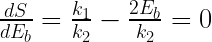
The maximum speed that a locomotive can attain with any given train occurs when the locomotive’s drawbar tractive effort exactly equals the rolling resistance of the train (see the Rolling Resistance page of this website).
The acceleration that a locomotive can achieve with any given train can be calculated by applying Newton’s Second Law of Motion – i.e. by subtracting the rolling resistance of the locomotive and train from the locomotive’s wheelrim tractive effort, and dividing the difference by the total mass of the locomotive and train.
Locomotive Power
Power is defined as “the rate of doing work”. Common units of power in the metric system are Watts (W), kilowatts (kW), Megawatts (MW) and Gigawatts (GW), where 1 Watt = 1 Joule per second = 1 Newton-metre per second. Alternative units of measurement are calories per second and kilo-calories per hour (1 kW = 860 kcal/hr) Common imperial units of power are: Btu per second (1 Btu/s = 1.06 kW) and the Horsepower where 1 (British) hp = 0.746 kW.
Power can also be defined as the multiple of force and speed, from which it can be deduced that a locomotive’s power and tractive effort (TE) are intrinsically related: Power = TE x speed.
Livio Dante Porta liked to define a locomotive’s power in the following thermodynamic terms, as can be found in his papers on “Fundamental Principles of Steam Locomotive Modernization and Their Application to Museum and Tourist Railways” and “Fundamentals of the Porta Compound System for Steam Locomotives“:
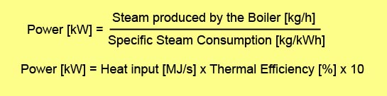
In reference to the first equation, Porta writes:
“Thus the power is limited by [the amount of steam supplied by] the boiler, while the function of the cylinders is to extract the maximum work from the steam supplied”,
“The second equation shows that the [power] limit is determined by the ability of the boiler to burn as much fuel per hour as possible, but the resulting power is determined by the thermal efficiency.”
A common point of confusion in locomotive terminology is the difference between indicated power and drawbar power, the basic difference being that “indicated power” is the power developed in the cylinders, whereas “drawbar power” is the power delivered at the drawbar. These terms are defined on separate pages.
The word “indicated” comes from the use of “Indicator Diagrams” that before the electronic era were mechanically plotted to indicate the variation in steam pressure inside a cylinder against the piston position as it sweeps through the piston over the length of its stroke. Separate diagrams for both ends of the cylinder were usually being plotted on the same sheet of paper.
The cylinder’s power output is calculated from the area contained within the plotted curve. Thus it can be deduced that a locomotive’s power output can be increased by increasing the area contained inside the Indicator Diagram.
An example of a typical Indicator Diagram (single ended) is shown below which also points out the four phases of the cylinder cycle:
-
Admission which occurs from the moment that the steam inlet port opens (near the beginning of the piston stroke) until the moment of “cut off” when it closes. At the beginning of the piston stroke, the cylinder pressure is (or should be) the same as the steam chest pressure. As the piston moves, some reduction of pressure may occur if the steam chest and/or the ports are too small.
-
Expansion which occurs from the moment of “cut off” until the exhaust port opens (near the end of the piston stroke). During this time, the steam in the cylinder expands adiabatically (meaning no heat input) resulting in the reduction of its pressure. The relationship between pressure and swept volume can usually be estimated using the equation PVn=K, where P is the steam pressure; V is the cylinder volume (including clearance volume); n is a constant, normally assumed to be 1.3 and K is a constant.
-
Exhaust which occurs on the return stroke between the moment the exhaust port opens until it closes again. During the exhaust phase, the cylinder pressure – or “back pressure” – is relatively constant, being governed by the steam flow through the exhaust ports and blast pipe. It can be readily seen that the area within the diagram can be dramatically increased by reducing the back pressure during the exhaust phase. This is the reason why simple modifications such as the fitting of double chimneys or Kylpor exhaust systems, result in immediate and dramatic improvement in locomotive performance.
-
Compression which occurs between the moment that the exhaust port closes until the inlet port opens. It is clear that the area within the Indicator Diagram can be maximised by making the exhaust phase as long as possible and the compression phase as short as possible. Some compression may nevertheless be desirable, as in the case of the 5AT where it provides “cushioning” for the pistons, counteracting the inertial forces that occur at the ends of each stroke and which would otherwise cause crank-pin overstress at very high speeds.

The shape of the indicator diagram and losses that are represented by it, are discussed on several separate pages including:
- Clearance Volume
- Wall Effects and Condensation
- Triangular Losses
- Incomplete Expansion
- Steam Tightness
Drawbar Power
The power output at the drawbar of a locomotive, the drawbar being the coupling between the locomotive and the train that it is hauling.
Drawbar power used to be measured by attaching a “dynamometer car” between the locomotive and its train. A dynamometer car incorporates a number of measuring devices including a calibrated spring for measuring the tractive force from the locomotive and a odometer wheel for accurately measurement of distance covered, and a timing device from which speeds can be calculated. In addition, the dynamometer car would house mechanical plotting devices and a team of people to monitor them. Nowadays an electronic load-cell can be fitted between the locomotive and its train and GPS used for measuring speed and distance, with data being logged and power outputs calculated on a laptop computer.
Drawbar power is the Indicated Power minus the mechanical losses in the locomotive’s motion and the rolling losses (including the wind losses) of the locomotive and its tender (see Resistance page). In the case of the 5AT, its drawbar power is diminished by the fitting of a large (80 tonne) tender. Because the rolling losses (and especially the wind losses) increase with speed, a locomotive’s drawbar power tends to peak at a lower speed than the Indicated Power.
Equivalent Drawbar Power
Equivalent drawbar power = drawbar power at constant speed on level tangent track. It eliminates the factors of acceleration and gradient/curvature resistance on the locomotive itself, the power to overcome which would be available at the drawbar at constant speed on level tangent track.
“Equivalent drawbar power vs. speed curves for various locomotives are shown below, copied from page 499 of David Wardale’s “The Red Devil and Other Tales from the Age of Steam” with the Tractive Effort curves removed for clarity.
[Note: The same diagram showing Tractive Effort vs. Speed can be viewed on the Tractive Effort page of this website.] [It is interesting to note that the Standard “Britannia” Class 7 produced a slightly higher power output than the Rebuilt “Merchant Navy” Pacific.]
Power-to-Weight Ratio
The Power-to-Weight ratio of a car is a measure of its ability to accelerate. A steam locomotive’s ability to accelerate is governed by its the ratio of its “power : total train weight” ratio and by its adhesive weight and adhesion coefficient (ignoring resistance factors).
The Power-to-Weight ratio of a steam locomotives is nevertheless an important meaure, however its implications are more nuanced than for a car. David Wardale explains the importance of having a high Power-to-Weight ratio on page 277 of his book as follows:
…. for high speed operation, a high Power : Weight ratio is essential. It implies the need for a small boiler, requiring highly efficient draughting, and high combustion rates, requiring an efficient combustion system. Failure to realize this means that at high speed most of a locomotive’s power is absorbed in pulling the locomotive itself. In fact any locomotive has a ‘zero drawbar power and thermal efficiency speed’ at which all its power is used to pull itself along, this speed being largely a function of its inbuilt power : weight ratio. That this ratio was not high enough in steam locomotives was the basic reason why steam was perceived as being unsuitable for the accelerated services which many railway administrations, especially in Europe, saw as essential if rail transport was to remain competitive. It was, however, only an inherent characteristic of most First Generation Steam (FGS) locomotives, not of steam traction per se.
On page 273 of his book he compares the Power-to-Weight ratio of the Red Devil with other FGS locomotives as follows:
The Drawbar Power-to-Weight ratio [of No 3450, the Red Devil] based on the engine weight only (i.e. excluding the tender) was 23.0 kW/ton calculated from the maximum recorded sustained equivalent drawbar power at 74 km/h, and 24.4 kW/ton based on the predicted maximum drawbar power at 100 km/h.
The maximum Drawbar Power-to-Weight ratio in kW per ton of engine weight for some other high power coal-fired locomotives were as follows:
- British Railways ‘Coronation’ class 4-6-2: 17.1 (best British figure based on transitory power)’
- German State Railways 45 class 2-10-2: 17.5 (approximate)1
- French National Railways 240P class 4-8-0: 23.3
- New York Central `Niagara’ class 4-8-4: 18.8 (representative of the very best American practice)
- Rio Turbio Railway 2-10-2: 20.6 (at 50 km/h, the maximum line speed)
- Porta’s experimental 4-8-0: 23.2
In respect of power capacity relative to size 3450 was therefore up to the best standards hitherto achieved despite it being a 2-cylinder simple expansion locomotive with moderate boiler pressure burning mediocre quality coal, this last factor being of great significance as very high power output from steam locomotives generally depended on burning high grade coal. Yet no-one should imagine that it represented a performance ceiling for the classical Stephensonian steam locomotive. Porta’s Second Generation Steam 2-10-0 proposal was designed to give a rated Drawbar Power-toWeight ratio of 32.5 kW/ton, and even with simple expansion 29 kW/ton should have been possible for a medium-speed machine if starting the design with a clean sheet of paper.
The predicted Drawbar Power-to-Weight ratio for the 5AT compared well with the above figures. With a maximum sustainable drawbar power at constant speed on level tangent track (and trailing a high capacity tender) of 1890 kW and an engine weight of 80 tons, its Drawbar Power-to-Weight ratio would have been 23.6 kW/ton.
[Note: Wardale uses the word “ton” to mean “tonne” in SI units.]
Steam Terms
Specific Steam Consumption
Specific Steam Consumption is defined as the steam consumed by a locomotive’s cylinders per unit output of power. It is typically measured in kg/kWh or kg/KJ.
A locomotive’s Specific Steam Consumption carries important implications as may be deduced from one of Porta’s favourite equations:

Thus for any given boiler output, a locomotive’s power can be increased by reducing its specific steam consumption – in particular, by increasing its cylinder efficiency and reducing steam leakage. Or as Porta put it, “the power is limited by [the amount of steam supplied by] the boiler, while the function of the cylinders is to extract the maximum work from the steam supplied”.
In Section 4 of his “Compounding” paper, Porta makes the observation:
“In steam locomotives, one should note that all the losses, except for incomplete expansion, are approximately constant for a given rotational speed. Hence, the aim is to have a longer cut-off but, given that this steeply increases the incomplete expansion losses, a compromise results at 20% to 30% (15% to 20% for the author’s proposals). Thus, the claims for poppet valves concerning their ability to work with very short cut-offs are illusory as they do not lead to low specific steam consumption because of these constant losses.
But there are economic reasons too. The Americans, who have the perverse habit of hooking as many cars as possible to their locomotives, force them to work at long cut-offs to get as high an α coefficient as possible so as to have a good use of the (expensive) adhesion weight. This of course leads to a high specific steam consumption, hence the need for massive evaporation, hence a massive boiler, hence idle axles to support a huge firebox, hence a gigantic tender, hence plants to supply coal en-route, hence immense coal stocks, hence diesel locomotives with a higher thermal efficiency (under test conditions) even if they cost twice as much and justify the Gulf War to supply them with oil.”
In the same paper, Porta also refers to Specific Steam Consumption in relation to the TE-Speed diagrams below, which appear under the heading “Boiler Size”. He introduces the diagrams as follows:
“The operating variables of any locomotive working with the throttle full open can be defined, for a fully warmed up condition, by (any) two of them. For example: tractive effort vs. speed; steam production vs. speed; cut off vs. speed, etc. In Fig. 32A, for example, the constant cut-off lines have been plotted on a TE vs. Speed diagram. There is a line corresponding to the maximum cut-off, and various lines for the various running cut-offs. As a first approximation, they are straight lines whose inclination is greater, the greater the imperfection of the internal streamlining. In ordinary locomotives in which the internal streamlining is poor, the lines have an envelope: no combination of speed and cut-offs make it possible to invade the zone M (Fig. 32B).
In Fig. 32A, the lines corresponding to constant evaporation have been drawn (lines 3) and also the lines for constant specific steam consumption (lines 5). They show a zone (hatched) in which this consumption is minimal (zone 6) and also a zone (zone 7 cross-hatched) in which it decreases (very much in the case of single expansion engines) due to the increase of the incomplete expansion losses. There is also a zone in which the various constant losses (leakage, wall effects) increase specific steam consumption – this is important in the case of shunting engines. Obviously, the aim of the designer is to provide a maximum area covered with consumptions differing as little as possible from the optimum.”
 Figs. 32A and 32B: Characteristic Lines
Notes on Fig 32: In Fig. 32A, Straight lines (1) are constant cut-off lines, (2) being the one corresponding to full gear. The various hyperbola-like lines (3) correspond to constant evaporation. Selecting one of them, such as (4) allows the provision of a definite boiler size. The hatched area (R) corresponding to the overload concept.
Curves (5) refer to constant specific consumption, the hatched area (6) indicating the combination of speed-tractive effort in which the consumption is at a minimum. Area (7) refers to low speed, low tractive effort characteristic of shunting services.
So far, the above refers to engines designed with good internal streamlining (a RARE case indeed!). Fig 32B is the common case in which the cut-off lines are so much inclined that they have an envelope (8): this corresponds to the American concept of “capacity power”; no combination of speed and tractive effort allows getting into the M region. Within the envelope area, the specific steam consumption is very high: this explains the huge size of American boilers and tenders.
Wardale also refers to Drawbar Specific Steam Consumption in his book, defining it (on page 273) as:

He goes on to point out that:
“Drawbar Specific Steam Consumption is therefore influenced by the power required to move the locomotive and as the measured values of this parameter were thought to be too high, the drawbar Specific Steam Consumption data [for the Red Devil] was distorted, especially at higher especially at higher speeds and lower steaming rates. (From this equation, it can be readily seen that the drawbar Specific Steam Consumption of a locomotive which was not capable of generating high power relative to its weight, was bound to suffer at high speed, however good the indicated Specific Steam Consumption was – e.g. Duke of Gloucester.”
In the Fundamental Design Calculations for the 5AT (see FDC 1.3), Wardale gives figures of minimum indicated Specific Steam Consumption for the Duke of Gloucester as 12.2 lb/hp-h and for the SNCF 141P Class 4-cyl. compound 2-8-2 as 11.2 lb/hp-hr, as compared to 11.24 lb/hp-h (= 5.1 kg/hp-hr or 1.9 kg/MJ) for the 5AT.
The Front-End Limit
As discussed on the Grate Limit page, the grate limit occurs when any increase in the rate of fuel delivery produces no increase in evaporation. In other words it represents the maximum rate of heat emission that a firebox can deliver beyond which point any additional fuel added to the firebox produces no additional steam.
The Front End Limit is a draughting limitation. In his paper titled “Two Point Four Pounds per Ton and The Railway Revolution“, Doug Landau defines the Front End Limit as occurring when the available excess air falls below about 20% [i.e. when] complete combustion can no longer be achieved. If this occurs prematurely, the locomotive concerned would be deemed a ‘poor steamer’. It could also be set by the designer at a value that would provide adequate steam, while at the same time avoiding ‘uneconomic’ combustion rates. The BR Standard locomotives were designed on this basis.
[In a letter to Chris Newman dated 10 Sep 2013, Dave Wardale wrote: The definition given by Doug Landau is correct, although it should be added that the cause of excess air falling to a useable limit is due to the blast pipe and chimney characteristic. Although BR claimed to have designed for this, Porta pointed out that whether the BR front end limit was by design or because they couldn’t do any better was an open question.]
In the same paper, Doug goes on to describe what he calls the “Discharge Limit” which he differentiates from the Front Edn Limit as follows:
Discharge Limit: This is also sometimes described as the ‘Front End Limit’, but it is quite different to the condition described above. It occurs when the steam exhaust velocity reaches the speed of sound. At this point theory has it that the pressure/draught relationship breaks down. Curiously however, there are recorded instances of this limit being exceeded without apparent distress. It does however involve very high back pressures upwards of 14 lbs/sq.in., and was definitely something best avoided.
Simple and Compound Expansion
The term “Simple Expansion” refers to the single use of steam in powering a steam engine. “Compound Expansion” refers to the multiple uses of steam in powering a steam engine.
In a “simple” engine, the steam enters the cylinder at high pressure, expands as it pushes the piston through its stroke, and is then exhausted to atmosphere as the piston returns, whereas in a “compound” engine, the exhausted steam is reused in a second “low pressure” cylinder where it expands further as it pushes the low pressure piston through its stroke. In the case of a double expansion compound, the steam will then exhausted to atmosphere. In a triple-expansion compound (mostly used in marine applications) the steam is reused again in a third (even lower pressure) cylinder.
In a compound engine, the steam will pass from the high pressure cylinder into a “receiver” (a pipe or pressure vessel of adequate volume) before being admitted into the low pressure cylinder. In some cases, the receiver will incorporate means of re-superheating the steam to raise its temperature to minimize the risk of condensation.
In historical texts, proponents of compound expansion are reputed to have claimed that greater use is made of the steam by expanding it twice (or more) thereby increasing the work it does and the efficiency achieved, whereas proponent of simple expansion are reputed to have claimed that the simplicity and lower cost of simple engines outweight the efficiency gains offered by compound expansion.
In fact the arguments for and against compound expansion are more complex – and too complex to expound on a website such as this and are more adequately covered elsewhere – for instance
- http://hubpages.com/hub/10-Advantages-of-Compound-Steam-Engine lists ten (easy-to-understand) advantages of compound expansion.
- Col. Roger’s biography of Chapelon also offers an excellent (and not overly technical) background on the subject; and
- Porta’s “Fundamentals of the Porta Compound System for Steam Locomotives” gives greater technical insight as explained further in the Compound Expansion page of this website.
However a few simple and pertinent points are worth summarizing here:
- Use of compound expansion allows longer cut-offs to be used, thereby delivering more uniform wheel-rim tractive effort;
- The ability of compound engines to operate efficiently at longer cut-offs increases their α-coefficient and thus their power-to-weight ratio.
- The reduction in vibration (or knocking) achieved from the use of longer cut-offs removes the incentive to operate a locomotive with a throttled (partially opened) regulator, thereby allowing full boiler pressure in the steamchest;
- More uniform torque delivered by compound locomotives reduces the propensity for initiation of wheel-slip at moments of (transient) peak torque. This renders compound locomotives better suited to heavy haulage;
- Reduced temperature differentials between steam entering and leaving a cylinder, minimizes heat losses and reduces or eliminates condensation, especially where the low-pressure steam is re-superheated.
Notwithstanding the above, Wardale has adopted simple expansion for the 5AT for several reasons. most of which are outlined in an FAQ on the subject:
- Wardale has no personal experience of compound locomotives to draw on or upon which to base an “assured” locomotive design;
- Wardale believes that for a high-speed locomotive such as the 5AT simple expansion – using all the cylinder refinements that are now possible, but which are not common knowledge – is the right choice, and that the 5AT will define ‘state of the art’ for 2-cylinder simple locomotives and may serve as a reference level to which the performance of all other types of locomotive (including compounds) can be compared.
- Such improvement in thermal efficiency that might be gained by compound expansion cannot guarantee to justify the extra design complexity and higher manufacturing costs involved.
- The limited low pressure cylinder volume possible within the British moving structure gauge, with a conventional layout of the cylinders, is an important limiting factor on compound design and performance.”
Steam Chest
The steam chest (or steamchest) is the “reservoir” for collection of steam as it passes between the superheater header and the inlet port to the cylinder.
The advantage of a large steam chest (as is the advantage of any reservoir) is that fluctions in pressure as the steam passes from the steamchest into the cylinder are reduced. The higher the steamchest pressure, the greater the quantity of steam that can be delivered to the cylinder while the inlet port is open, and the higher the cylinder pressure at the point of cut-off. Maximizing cylinder pressure at the point of cut-off serves to maximize the work done by the steam on the piston. In alternative words, it serves to maximize the area within the indicator diagram.
Ideally, the steamchest volume should equal (or exceed) the cylinder volume, but never came near this in FGS locomotives. One of the modifications that Wardale made in developing The Red Devil was enlargement of the steam chests which are easily visible on the photo below. In fact, the extent of the enlargement was limited by other constraints such that their volume increased only from 33.2% of cylinder volume to just 35.5% compared to an ideal minimum of 100%. By contrast, the 5AT steam chest volume is almost exactly 100% – see line [158] of FDC 6.


Dave Wardale defined Equivalent Evaporation as follows:
Equivalent evaporation = evaporation from and at 100°C. Evaporation figures thus expressed eliminate the effects of different feedwater and superheat temperatures, and are therefore a true measure of comparison between different boilers. [Letter from Dave Wardale to Chris Newman, 5th April 2001.]
Equivalent Evaporation might be more simply defined as “the quantity of water at 100°C that a boiler can convert into dry/saturated steam at 100°C from each kJ of energy that is applied to it. This defines it in terms of kg (of water/steam) per kJ of energy. However it is sometimes defined in units of kg water per kg of fuel, and (as in the case of the graph above) kg water/steam per hour.
On page 79 of his book “Red Devil and Other Tales from the Age of Steam”, Wardale includes the graph copied below which illustrates the difference between actual evaporation and equivalent evaporation (applying to an SAR Class 25 4-8-4).

A more exact definition of Equivalent Evaporation in units of kg/hr comes from “Thermal Engineering” pages 608/9 by R.K. Rajput (see Google Books):
“Generally the output or evaporative capacity of the boiler is given as kg of water evaporated per hour but as different boilers generate steam at different pressures and temperatures (from feed water at different temperatures) and as such have different amounts of heat ; the number of kg of water evaporated per hour in no way provides the exact means for comparison of the performance of the boilers. Hence to compare the evaporative capacity or performance of different boilers working under different conditions it becomes imperative to provide a common base so that water be supposed to be evaporated under standard conditions. The standard conditions adopted are: Temperature of feed water 100°C and converted into dry and saturated steam at 100°C. As per these standard conditions 1 kg of water at 100°C necessitates 2257 kJ (539 kcal in MKS units) to get converted to steam at 100°C.
“Thus the equivalent evaporation may be defined as: the amount of water evaporated from water at 100°C to dry and saturated steam at 100°C.
“Consider a boiler generating ma kg of steam per hour at a pressure p and temperature T.
Let h = Enthalpy of steam per kg under the generating conditions.
-
- h = hf + hfg ……. Dry saturated steam at pressure p
- h = hf + xhfg ……. Wet steam with dryness fraction x at pressure p
- h = hf + hfg + cp (Tsup – Ts) ….. Superheated steam at pressure p and temperature Tsup
- hf1 = Specific enthalpy of water at a given feed temperature.
Then heat gained by the steam from the boiler per unit time = ma x (h – hf1)
The equivalent evaporation (me) from the definition is obtained as:
The evaporation rate of the boiler is also sometimes given in terms of kg of steam /kg of fuel. The presently accepted standard of expressing the capacity of a boiler is in terms of the total heat added per hour.
An alternative definition is offered by Applied Thermodynamics by Onkar Singh as follows:
“For comparing the capacity of boilers working at different pressures, temperatures, different final steam conditions etc, a parameter called “equivalent evaporation” can be used. Equivalent evaporation actually indicates the amount of heat added in the boiler for steam generation. Equivalent evaporation refers to the quantity of dry saturated steam generated per unit of time from feedwater at 100°C to steam at 100°C at the saturation pressure corresponding to 100°C. Sometimes it is called equivalent evaporation from and at 100°C. Thus mathematically it could be given as:

For a boiler generating steam at ‘m’ kg/h at some pressure ‘p’ and temperature ‘T’, the heat supplied for steam generation = m x (h – hw), where h is the enthalpy of final steam generated and hw is enthalpy of feedwater. Enthalpy of final steam shall be:
-
- h = hf + hfg = hg for final steam being dry saturated steam (hf, hfg and hg are used for their usual meanings),
- h = hf + x . hfg for wet steam as final steam,
- h = hg + cp sup.steam . (Tsup – Tsat) for superheated final steam.
Equivalent evaporation (kg/kg of fuel) =

Equivalent evaporation is thus a parameter which could be used for comparing the capacities of different boilers.”
Note – the last equation purports to express equivalent evaporation in units of kg/kg of fuel, but in fact the units are actually in kg/hr.]
Superheating of Steam
Page Under Development
This page is still “under development”. Please contact Chris Newman at webmaster@advanced-steam.org if you would like to help by contributing text to this or any other page.’
Background
On page 160 of his book “The Red Devil and Other Tales from the Age of Steam” Wardale confirms that:
“The fundamental laws of thermodynamics dictate that for the maximum thermal efficiency from any heat engine, the working fluid must commence its expansion from the highest possible temperature. In a steam locomotive this was accomplished by superheating the steam.”
He goes on to explain that superheating not only improves the ideal (Carnot) cycle efficiency but also gives other practical benefits not connected with the Second Law of Thermodynamics (and not often appreciated), such as:
-
Reduced heat transfer losses (condensation) to the cylinder walls,
-
Reduced steam flow pressure drop for a given volumetric flow rate, and
-
Reduced water consumption.
He goes on:
“Such was the benefit of the Schmidt type superheater realized in actual service that it must rank as the twentieth century’s most important single contribution to the art of steam locomotive design. Yet as with the exhaust system and feedwater heating, superheating was rarely fully exploited. The superheat temperature should have been the maximum possible – full stop – and this should have been all the motivation that was needed to improve the factors such as valve and cylinder lubrication which were said to be limiting it.
However all too often the reverse attitude seems to have been taken, these factors being seen as rigid barriers to higher temperatures and lower-than-possible ones being consequently accepted as the highest that could be allowed – or simply ‘good enough’. This was certainly the case on, for example, the SAR, where it was thought that steam temperatures of the order of 380°C as transitory values were all that were possible due to the lubrication issue. Worse still, the myth that high superheat merely wasted energy in the exhaust steam was believed by not a few engineers right down to recent times. On the other hand both Germany and France pursued means to allow the use of high steam temperatures: 400°C was normal in Germany on the standard designs first introduced in 1925 whilst Chapelon’s locomotives recorded temperatures as high as 425°C.”
Technical Outline
Superheating is achieved by passing saturated steam from the “main pipe” through small diameter tubes called superheater elements which are placed inside large diameter boiler tubes called superheater “flues”. Combustion gases passing through these flues transmit their heat to the steam raising its temperature above (usually far above) its saturation value.
Superheater elements are connected to a superheater header – a small steam reservoir that is separated into two chambers. One end of each superheater element is connected to one of these chambers, and the other end to the second chamber. Saturated steam from the boiler enters the “saturated steam chamber” from where it passes through any one of the superheater elements and thence back into the second “superheated steam chamber” of the header. From there is passes through steam pipes to the steam chests and thence to the cylinders.
The steam regulator (or “throttle” as Wardale prefers to call it*) may be located on either side of the superheater header. In the case of the 5AT, the throttle is placed on the superheated steam side of the header.
[* Wardale prefers to use the term “throttle” because it better describes the action operating a locomotive with a partially-opened regulator.]
The picture below (of the sectioned Merchant Navy Pacific 35029 housed in the National Railway Museum in York) illustrates the arrangement of superheater flues, elements and header.

An alternative view, copied from a 1930s children’s book, shows the main steam pipe that delivers saturated steam to the superheater header. [Of interest is the steam collection pipe at the highest point of the domeless Belpaire (LMS) boiler.] Click on image to see full-size enlargement.

See also:
Note: In relation to the application of Feedwater Heating to “The Red Devil“, Wardale points out that “the need to increase the superheat on the modified 25NC was clear: not only was the existing steam temperature too low but the use of a feedwater heater always decreased the superheat and this factor had to be compensated for”.
This non-intuitive observation is explained in a footnote to a transcription of the text from the book which is summarized as follows: “Since less heat needs to be generated in the firebox to boil preheated water, then there’ll be less heat available for superheating the steam that is generated”.
Drafting & Combustion
The Grate Limit as it relates to Boiler Efficiency
On page 78 of his book The Red Devil and Other Tales from the Age of Steam, Dave Wardale defines the Grate Limit for a (normal) locomotive firebox as follows:
The grate limit is the point “at which even by firing more coal and supplying more combustion air, no more steam could be produced.”
Put another way, it is the point at which the rate of firing fuel into the firebox exactly equals the rate at which unburned fuel is carried out of the firebox by entrainment in the combustion air.
Wardale quotes an equation derived by L.H. Fry in 1924 that (effectively) relates the grate limit to boiler efficiency as follows:
Eb = k1 – k2 x M/G, where
- Eb = Boiler Efficiency
- M = Firing Rate
- G = Grate Area
- k1 = predicted boiler efficiency at zero firing rate
- k2 = the slope of the graph relating boiler efficiency to firing rate.
The equation is illustrated in graphical form below (Fig 20 in Wardale’s book):
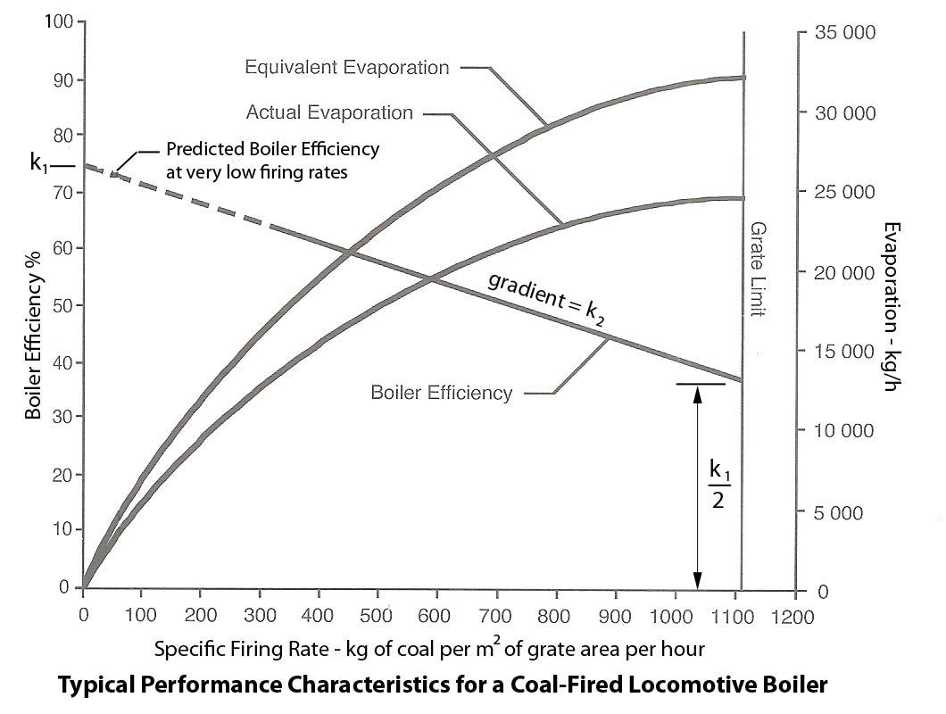
The above equation is empirical, yet it is one that produces a fascinating insight – namely that the boiler efficiency at the grate limit is exactly 50% of the predicted efficiency at zero firing rate.
In the diagram, k1 is the maximum predicted boiler efficiency (at zero firing rate) and k2 is the slope of the straight line relating efficiency to firing rate. [A simple mathematical proof that (based on Fry’s equation) the boiler efficiency at the grate limit is exactly half the maximum efficiency is given further below. A definition of Equivalent Evaporation is also provided on a sepate page.]
Wardale goes on to demonstrate that Fry’s equation represents reality, being demonstrated in a boiler test conducted on a Pennsylvania Railroad M1a 4-8-2 locomotive. Here Wardales adjusts his definition of the grate limit as follows:
The grate limit was the point at which “the heat liberation rate in the firebox was a maximum, which for all practical purposes occurred when the fuel entrained in the draught and escaping unburnt equalled the amount of fuel actually burned, this point being linked to the start of gross firebed fluidisation.”
In other words, the grate limit is reached when half the fuel that is fired into the firebox escapes from the chimney. He illustrates this with the diagram below taken from Fig 21 on page 80 of his book, to which the percentage figures on the right have been added [including an approximate division of “evaporation” into latent and sensible heat]:
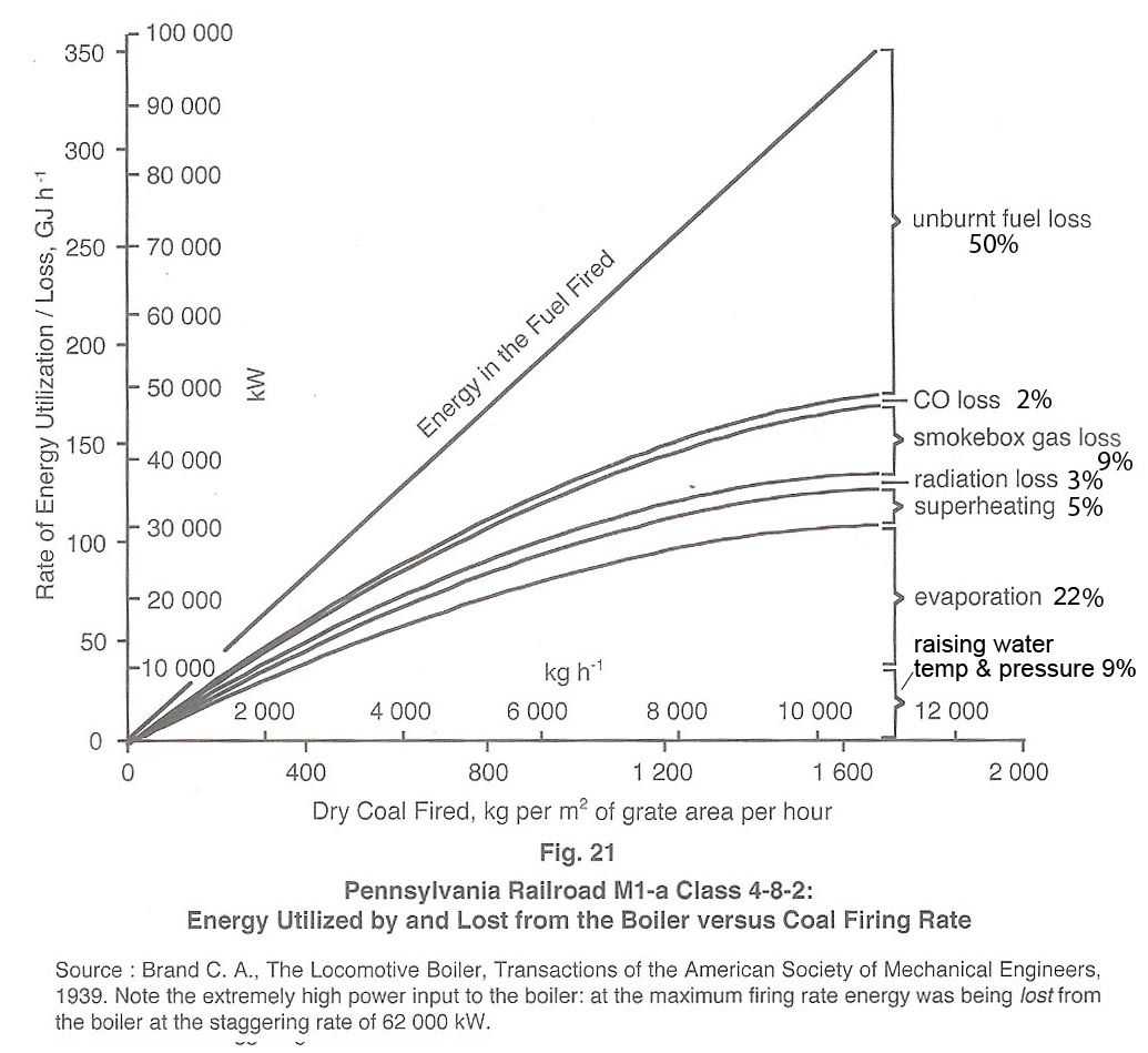
It should be noted that Fry’s equation does not hold for GPCS fireboxes. Indeed, the fact that it does not hold is one of the great advantages that GPCS fireboxes offer.
A simple mathematical proof that, based on Fry’s equation, boiler efficiency at the grate limit is exactly half the maximum efficiency, is as follows:
Fry’s Equation: Eb = k1 – k2 x M/G, where:
- Eb = Boiler Efficiency
- M = Firing Rate
- G = Grate Area
- k1 = predicted boiler efficiency at zero firing rate
- k2 = the slope of the graph relating boiler efficiency to firing rate.
Boiler efficiency may also be defined as the amount of energy released from the boiler in the form of steam divided by the amount of energy released in the firebox from the fuel.
Thus if the Steaming Rate = S, then Eb = S ÷ M/G
Thus M/G = S/Eb
Substituting this in Fry’s equation we get: Eb = k1 – k2 x S/Eb
from which: Eb2 = k1.Eb – k2.S and thus: S = k1.Eb/k2 – Eb2/k2
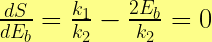
From calculus, we know that S reaches a maximum (or minimum) when the slope of the curve = zero. This occurs when
i.e. when …..

Thus the maximum steaming rate occurs at the point where the boiler efficiency is half the predicted value at zero firing rate.
The Front-End Limit
As discussed on the Grate Limit page, the grate limit occurs when any increase in the rate of fuel delivery produces no increase in evaporation. In other words it represents the maximum rate of heat emission that a firebox can deliver beyond which point any additional fuel added to the firebox produces no additional steam.
The Front End Limit is a draughting limitation. In his paper titled “Two Point Four Pounds per Ton and The Railway Revolution“, Doug Landau defines the Front End Limit as occurring when the available excess air falls below about 20% [i.e. when] complete combustion can no longer be achieved. If this occurs prematurely, the locomotive concerned would be deemed a ‘poor steamer’. It could also be set by the designer at a value that would provide adequate steam, while at the same time avoiding ‘uneconomic’ combustion rates. The BR Standard locomotives were designed on this basis.
[In a letter to Chris Newman dated 10 Sep 2013, Dave Wardale wrote: The definition given by Doug Landau is correct, although it should be added that the cause of excess air falling to a useable limit is due to the blast pipe and chimney characteristic. Although BR claimed to have designed for this, Porta pointed out that whether the BR front end limit was by design or because they couldn’t do any better was an open question.]
In the same paper, Doug goes on to describe what he calls the “Discharge Limit” which he differentiates from the Front Edn Limit as follows:
Discharge Limit: This is also sometimes described as the ‘Front End Limit’, but it is quite different to the condition described above. It occurs when the steam exhaust velocity reaches the speed of sound. At this point theory has it that the pressure/draught relationship breaks down. Curiously however, there are recorded instances of this limit being exceeded without apparent distress. It does however involve very high back pressures upwards of 14 lbs/sq.in., and was definitely something best avoided.
Primary and Secondary Combustion Air and Combustion Gases
Combustion Air is the air drawn through the firebox by the draughting system which allows combustion to take place. Only the oxygen content of the air (approx 18%) is used in the combustion process, the remainder (mostly nitrogen) being inert and serving no function other than wasting energy and cooling the fire.
Combustion Air comes in two forms:
- Primary Combustion Air which is drawn upwards through the ashpan, grate and firebed, and
- Secondary Combustion Air which is drawn in over the top of the fire – e.g. through the firehole door.
Essentially, the primary air releases heat from the fuel and the secondary combustion air releases heat from volatile gases released from the hot coal in the firebed. The chemical reactions that release heat from the fuel are sometimes complex, but the end-product is a combination of carbon dioxide gas and water vapour mixed with small quantities of carbon monoxide and oxides of other impurities (plus large volumes of nitrogen). These reaction products are termed Combustion Gases.
The quantity of combustion gases released from the firebox can be much larger than the volume of steam exhausted from the cylinders. For instance at the 5AT’s maximum designed drawbar power (1800 kW at 113 km/h), Wardale calculated that the mass of combustion gas ejected through the chimney would be 2.2 times the mass of steam passing through the blast nozzles.
In normal steam locomotive operation, the bulk of combustion air is drawn through the ashpan and grate, thus being classified as “primary air”. Secondary air is normally only available when the firehole door is opened, usually for firing and occasionally for more extended periods to burn off volatile material and thus reduce smoke emissions.
The Gas Producer Combustion System (GPCS), as described elsewhere on this website, involves a continuous flow of secondary air, usually through ducts passing through the outer and inner firebox sides and crown, and corresponding reduction in primary air.
To reduce temperature drop in the firebox, it is possible to preheat the air before it is mixed with the fuel, however the first time this advance was ever implemented in practice was by David Wardale in the development of a modernized design of the QJ 2-10-2 freight locomotive. Wardale never complete the final design for this machine, but one locomotive – QJ No 8001 – was modified by being fitted with an experimental heat exchanger for the heating combustion air. The photo below of the modified machine has been copied from Hugh Odom’s Ultimate Steam website.

To be continued ….
Locomotive Exhausts
Page Under Development
This page is still “under development”. Please contact Chris Newman at webmaster@advanced-steam.org if you would like to help by contributing text to this or any other page.’
Background
A steam locomotive’s exhaust system is perhaps the most innovative of all the ideas that underpin the “Stephensonian” concept. It’s cleverness derives from its automation whereby the draught that provides the oxygen to generate heat from the fire is automatically governed by the work that the engine is doing. The harder it steams, the greater the exhaust and thus the greater the draught and greater the heat produced.
In his introduction to FDC 12, Wardale describes the exhaust system (as it relates to the 5AT) as follows:
“The exhaust system, dynamically connecting the boiler and cylinders, is thermodynamically the heart of the locomotive and must therefore be as good as possible within practical limitations. That the exhaust entrains sufficient combustion air to sustain the combustion rate necessary to match the steam demand throughout the boiler’s evaporative range is a cardinal point for good performance from any steam locomotive, and that it does this with the minimum of exhaust steam energy is the key to optimum performance. This point is especially important on the 5AT as the locomotive is to operate mostly at high speed with full throttle and low cut-off, giving high heat conversion to mechanical work in the cylinders and therefore limiting the amount of energy available for draughting work in the exhaust steam (it is common for locomotives to steam adequately at long to medium cut-offs but not at short, for this reason), and this is compounded on the 5AT by the use of piston valves with exhaust lap, delaying release.”
In most First Generation Steam (FGS) locomotives, the exhaust system was developed largely through rule of thumb with very little application of scientific or engineer theory. Exhaust steam from the cylinders passes through passages (usually cast into the smokebox saddle) which meet below a blast nozzle through which the steam is ejected upwards through a “petticoat” mounted under the chimney, the petticoat acting as a venturi that creates a partial vacuum inside the smokebox that draws combustion gases from the firebox and mixes it with the exhausting steam. The size of blast nozzle and the geometric arrangement of the nozzle and petticoat were critical in obtaining a good draught and therefore good steaming – a smaller nozzle causing greater exhaust pressure which creates a greater blast and thus a greater vacuum and draught.
A typical FGS arrangement is shown in the cut-away drawing below copied from a 1930s children’s book. Click on image to see full-size enlargement.
Relationship between Exhaust Pressure and Power Output
Improving a locomotive’s steaming by reducing its blast pipe diameter and thereby increasing its exhaust pressure, has a very serious and measurable effect on a locomotive’s power output. Conversely, fitting an improved exhaust system that maintains smokebox vacuum when using of a larger blastpipe orifice, can significantly boost a locomotive’s power output or reduce its fuel and water consumption at a given power output.
The benefit derived from an improved exhaust with enlarged blastpipe can readily be seen by inspecting a typical indicator diagram and bearing in mind that the area contained within its curve represents the power delivered by the cylinder. The hypothical (simplified) diagram below, plotted using an Excel spreadsheet, illustrates a 14% increase in power output resulting from a reduction in exhaust pressure from 75 kPa (10.9 psi) down to 25 kPa (3.6 psi).

The “Double Chimney”
During the 1950s, the double chimney was seen in Britain to be a major technological advance bringing significant performance improvements to older designs such as the Kings and Castles from the GWR. The basic aim was to increase the blast pipe nozzle area through the use of two nozzles each exhausting through its own petticoat venturi, thereby reducing cylinder back pressure and increasing power output without loss of draught (or alternatively, increasing draught without loss of power).
Unfortunately, it seems that when exhaust system improvements were being planned for post-war locomotives in the UK, too little attention was paid to earlier developments that had taken place in France where in 1926 André Chapelon had developed a much more sophisticated and scientifically-based exhaust system design that he called the “Kylchap” in recognition of a Finnish engineer by the name of Kyösti Kylälä on whose ideas Chapelon had based his design. In fact, in 1938 Gresley fitted Kylchap exhausts to four of his then new A4 locomotives, one of which (Mallard) demonstrated its superiority by achieving the world speed record for steam. Presumably it was the financial constraints of the notoriously cash-starved LNER that deterred the widespread fitting of Kychap exhausts to other members of the class until the 1950s, by when they had become part of BR’s fleet. It is to be regretted that Kylchap exhausts were not more widely used since the performance benefits and fuel cost savings that they offered must have outweighed their capital cost many times over.
Modern Developments – The Kylchap, Kylpor and Lempor Exhausts
For further discussion of modern steam exhaust systems, including the Kylchap, Kylpor and Lempor, see the Exhaust Systems page of this website under Principles of Modern Steam.
A theoretical minimum amount of oxygen is needed to react with the combustible elements (mainly carbon and hydrogen) in a given quantity and type of fuel. In practice an additional (or excess) quantity of air is required to ensure adequate contact between fuel and oxygen to guarantee efficient combustion. There are no hard-and-fast rules defining the amount of excess air that is required in any given situation, but 20% is a generally accepted minimum. For instance, in his paper “Two Point Four Pounds per Ton and The Railway Revolution“, Doug Landau defines the Front End Limit as occurring “when the available excess air falls below about 20% [i.e. when] complete combustion can no longer be achieved”.
The quantity of air – and therefore the quantity of excess air – passing through the firebox is governed by the smokebox vacuum and the flow resistance through the ashpan, firebox and boiler tubes/flues. Thus the quantity of excess air passing through the firebed is dependent on the smokebox vacuum and therefore the exhaust system performance. In the normal situation, where 100% of combustion air passes through the firebed, increasing the excess air is likely to result in fuel loss caused by the entrainment of coal particles that are carried away with the combustion gases. However where GPCS is applied, only a small proportion of the combustion air (perhaps 30%) passes through the firebed, thereby allowing much higher levels of excess air to be applied.
Fig 27 from Wardale’s book “The Red Devil and Other Tales from the Age of Steam” illustrates the reduction in fuel carry-over that can be achieved with GPCS, from which the possibilities for increased airflow may be deduced. 
As might be expected, increasing the amount of excess air above the 20% nominal minimum has the beneficial effect of reducing smoke emissions, however it penalizes performance because the higher gas flow through the firebox and boiler require the exhaust system to work harder, thereby raising cylinder back-pressure. Wardale also points out (in a letter to Chris Newman dated 5 Apr 2001) that “loss of heat from excessive amounts of air can be far greater than that carried away in soot (smoke)”. He followed this up in a second letter with the observation that “excess air should be kept to a minimum for best boiler efficiency …. Diluting of pollutants [is] a worthy goal [but] I would go for both.”
In his design for the 5AT exhaust system, Dave Wardale opted for 30% excess air at maximum firing rate, saying that “this is a ‘safe’ value. The [oil fuel] combustion equipment must be designed to allow adequately complete combustion with the minimum of excess air.” In his combustion calculations (FDC 11.2 item 17) he adds that: “from experience [30% excess air] is an appropriate value for locomotive operation at maximum evaporation, when the combustion time is extremely short. A general goal is the highest combustion efficiency with the lowest excess air, and if the combustion equipment can give adequately complete combustion with lower excess air then boiler efficiency will be higher”
Mechanical Terms
Tractive Effort
“Tractive effort” (TE) is the force applied by a locomotive for moving itself and a train. Tractive effort or tractive force is measured in kilo-Newtons (kN) or pounds force (lbf) where 1 kN = 228.4 lbf.
As with “power”, there are different methods of measuring tractive effort:
- Drawbar tractive effort – the force applied by a locomotive to the connection to its train. If the locomotive is running light (with no train) then its drawbar TE = 0.
- Wheel-rim tractive effort – the force applied by a locomotive to the rails through its driving wheels. The difference between Wheel-rim TE and Drawbar TE is the force required to move the locomotive in overcoming internal (mechanical), rolling and wind resistances.
- Indicated or Cylinder tractive effort – a hypothetical force estimated by adding to the Wheel-rim TE the force required to overcome the frictional resistance of piston against cylinder, piston-rod against gland, crosshead against slidebar and the rotational resistance of big and small-end bearings. In the case of the 5AT (FDC 1.1 lines 46 and 47), the Wheel-rim TE is estimated to be 93% of Cylinder TE at starting and 96% when running.
- Starting tractive effort – the pulling force exerted by a locomotive when starting from rest.
The commonly used formula for calculating a locomotive’s starting Tractive Effort is
The above formula is simplified in that it takes no account of the piston rod diameter which reduces the effective area of (and therefore the force applied to) the rear side of the piston. In the case of the 5AT (and a few other locomotive types) the presence of a tail-rod reduces the effective area of both sides of the piston. [Thanks to Larry Dean for drawing my attention to an error in the formula which is now corrected.]
A locomotive’s starting tractive effort only provides an indication of the size of train that it can start. It does not measure the ability of the locomotive to pull a train at speed. This is because tractive effort reduces as speed increases. A locomotive that can maintain a high tractive effort at speed is a more “powerful” locomotive than one that cannot since Power = Tractive Force x Speed.
The relationship between TE and Speed for a variety of locomotives is illustrated in the diagram below (copied from page 499 of Wardale’s book “Red Devil and Other Tales from the Age of Steam“) in which it can be seen that the TE of the “Super Class 5 4-6-0 (5AT) remains higher than even the most powerful British Pacifics once their speed exceeds 70 km/h. The 5AT’s ability to maintain high TE at speed is a measure of its ability to deliver and make use of steam that is supplied to the cylinders i.e. “good breathing”. (The diagram can be compared to the Power – Speed diagram copied from the same page, which is shown on the Drawbar Power page of this section of the website.)
It should be noted that the actual wheel-rim tractive effort of a locomotive varies considerably as the wheels rotate. This variation is most pronounced in two and four-cylinder machines with cranks set 90 degrees apart. When one piston is at mid-stroke where it generates maximum torque, the second piston is at front or back dead centre where it provides zero torque. The maximum starting torque is half what you’d get if both pistons were acting in unison – hence the factor 2 in the bottom line of the equation.
Calculation of tractive force is further complicated by changes in crank angle as the wheels rotate and by the variation in piston force resulting from “cut-off” and the subsequent expansion of the steam in the cylinder. This can be seen in the diagram below showing the variation in tractive force as calculated for the 5AT, at starting, at max drawbar-power output and at maximum speed. It also compares the starting the nominal starting tractive effort when new and when wheels and cylinders are part worn (both of which result in an increase in TE).
A locomotive’s tractive effort (at all speeds) is limited by its adhesive weight and the available coefficient of adhesion between wheel and rail, as illustrated in the above diagram and as discussed in more detail on the Adhesion page of this website.
The maximum speed that a locomotive can attain with any given train occurs when the locomotive’s drawbar tractive effort exactly equals the rolling resistance of the train (see the Rolling Resistance page of this website).
The acceleration that a locomotive can achieve with any given train can be calculated by applying Newton’s Second Law of Motion – i.e. by subtracting the rolling resistance of the locomotive and train from the locomotive’s wheelrim tractive effort, and dividing the difference by the total mass of the locomotive and train.
Adhesion and Adhesive Weight
Adhesion is the frictional resistance that prevents a locomotive’s driving wheels from slipping on the rail. Available adhesion depends on the conditions of both the rail and the wheel. With a clean dry wheel running on a clean dry rail the “frictional coefficient” between them may be as high as 0.35 or 35%. The presence of oil and other contaminents may reduce it to near zero.
Adhesive Weight is that part of a locomotive’s weight that is supported by its driving wheels. In the case of modern Bo-Bo and Co-Co diesels and electrics, 100% of their weight is supported by their driving (or driven) wheels which allows them to deliver a very large starting Tractive Effort. The same applies to 0-6-0T steam engine, however with 0-6-0 tender engines, perhaps no more than 70% of its total weight may be supported by its drivers. The greater the number of carrying wheels, the less weight is available for adhesion, and in the case of a typical Pacific locomotive less than 50% of total weight may be available for adhesion. This has serious consequences in terms of limiting the locomotive’s wheel-rim tractive effort and its drawbar power.
Coefficient of Friction is defined as the frictional resistance between two bodies and the “normal” force applied between them. In the case of a locomotive, the Frictional Coefficient = available frictional resistance ÷ adhesive weight on the driving wheels.
Adhesion Factor is the inverse of Friction Coefficient, i.e. Adhesion Factor = adhesive weight on the driving wheels ÷ available frictional resistance.
Frictional Coefficient between Wheels and Rail: A clean dry wheel on a clean dry rail may have a coefficient of friction as high as 0.35 or 35% at zero speed. This can drop to 0.25 in wet conditions, and very much lower if the rail is contaminated with lubricating substances such as ice, oil and leaves.
However the frictional coefficient between wheel and rail is not constant: due to “elastic slip” it falls as speed rises which is why wheel slip can (and does) occur at speed. Curves showing the relationship between speed and friction coefficient are shown below (taken from Koffman’s equations):

Estimating a locomotive’s adhesion limit is further complicated by the fact that its wheel-rim tractive effort varies considerably over each wheel revolution, even at high speed. As a result, momentary slipping can occur where the tractive force peaks and this can, in unfavourable circumstances, initiate full-scale slip at low and high speeds.
For further information, see the Advanced Adhesion page in the Principles of Modern Steam section of this website.
For a comprehensive dissertation on the subject, see A Selection of Papers by L.D. Porta Volume 2.
Locomotive and Train Resistance
A locomotive’s tractive force is required to overcome the resistance to motion of both locomotive and train. When the tractive force is greater than the resistance, then the train will accelerate in accordance with Newton’s law of motion: Force = Mass x Acceleration or Acceleration = Force ÷ Mass. If the tractive force is equal to the resistance, then the train will travel at constant speed. If the tractive force is less than the resistance, then the train will slow down.
There are various forms of resistance that need to be considered.
Locomotive Resistance
-
Starting resistance, associated with static friction which is usually higher than dynamic friction – i.e. it needs to be overcome before the locomotive will start moving;
-
Internal (mechanical/frictional) resistance from the locomotive’s motion etc;
-
Rolling resistance deriving from axle bearings and wheels on rail – it increases in proportion to the speed;
-
Wind resistance increases in proportion to the square of the speed;
-
Gravitational resistance when on an incline – equals the locomotive weight x the gradient;
-
Rail curvature resistance applies only to curved track – being proportional to the curvature of the track (or inversely proportional to the radius of curvature).
Train Resistance
-
Starting resistance, associated with static friction which is usually higher than dynamic friction – i.e. it needs to be overcome before the train will start moving. In the case of roller bearing stock, this value is close to zero, but can be significant where journal bearings are fitted to wagons;
-
Rolling resistance deriving from axle bearings and wheels on rail – it increases in proportion to the speed;
-
Wind resistance increases in proportion to the square of the speed;
-
Gravitational resistance when on an incline – equals the train weight x the gradient;
-
Rail curvature resistance – being proportional to the curvature of the track (or inversely proportional to the radius of curvature), but applying only to the length of train on the curved track.
In addition, inertial resistance has also to be considered (e.g. when a train is being accelerated).
The term “specific resistance” means the resisting force per tonne of (train) weight. It is pertinent to note that the specific resistance of empty freight trains and of passenger trains is much higher than that of loaded freight trains. This is largely because the wind resistance of an empty or lightly loaded train is the same as or higher (see below) than that of a full train. Since the wind resistance becomes dominant at higher speeds, the total resistance per tonne of train weight becomes higher. In the case of open-topped wagons, the wind resistance of empty wagons is higher than of full wagons because of the increased in air turbulence inside and around the empty wagon bodies. This is illustrated in the graphs at the bottom of this page.
It might also be mentioned that wind resistance is higher when the wind comes from an angle to the direction of the train than when the wind is directly head-on to the train. This is because the wind has more impact on the ends of each wagon or carriage than when the wind is directly in front of the train where slipstreaming from one wagon or carriage to the next reduces drag.
Train resistance can be measured by the force in the coupling connecting the locomotive to its train (e.g. using a dynamometer car, or in latter days using an electronic load cell). Locomotive rolling resistance is harder to measure.
There are no exact methods for estimating locomotive or train resistance and reliance has to be placed on empirical formulae based on measured values. Almost every country’s railway has its own formulae for estimating rolling resistance, all (presumably) being based on recorded measurements.
Most resistance formulae are divided into three sections:
-
a fixed constant, representing a fixed part of the rolling resistance,
-
a term proportional to the train speed, representing a variable part of the rolling resistance, and
-
a term proportional to the square of the train speed representing wind resistance.
One of the more recent national train resistance formula to be developed was the Serbian one that was formulated in 2005 based on tests undertaken by M. Radosavljevic from the Department of Mechanical Engineering, the Institute of Transportation in Belgrade. He wrote a paper on his findings entitled “Measurement of Train Traction Characteristics” published in the Proceedings of the Institution of Mechanical Engineers Vol 220 Part F: J. Rail and Rapid Transit. A copy of the formulae and their graphical representation is copied below. (See below for further comparisons)
 The above formulae are compared with additional train resistance formulae in the Excel graph below [click on the image for a full-sized PDF image.] The additional formulae covered are as follows
-
China National Railways (full wagons)
-
China National Railways (empty wagons)
-
Canadian National Railway (full wagons)
-
An (unnamed) Australian mineral railway (full wagons)
-
An (unnamed) Australian mineral railway (empty wagons)
-
Koffman’s formula for BR carriages as used by Wardale in FDC 1.1.
It will be readily seen that (as explained above) the specific resistance of empty wagons is much higher than that of full wagons and that for BR Carriages is also high by comparison with loaded wagons (due to their relatively light loaded weight). On the other hand the majority of formulae give very similar estimates for the specific rolling resistance of full wagons, with the exception of the (unnamed) Australian mineral railway figures which show much lower figures. This is probably because the wagons are much larger and more heavily loaded than those in the other countries listed.
Wardale’s Resistance Calculations
In FDC 1.1 (line 24) and FDC 1.2 (line 2) Wardale uses the following formulae for calculating locomotive and carriage rolling resistence (respectively):
-
Locomotive rolling resistance: R ≈ (45 + 0.24v + 0.0036v2) N/Tonne
-
Carriage rolling resistance: R = (1.1 + 0.021v + 0.000175v2) kg/tonne – from Koffman applying to BR coaches.
where R is the specific rolling resistance in N/Tonne of weight and v = speed in km/h.
-
In FDC 1.3 line 164, Wardale quotes Koffman to assume a specific starting resistance on level tangent track for roller bearing stock of 7.0 kg/tonne (= 6.99 N/kN).
-
In FDC 1.3 line 166, Wardale uses a figure of 100 N/tonne (=10.2 N/kN) for the specific starting resistance for a locomotive.
Chinese National Railways Resistance Calculations
For the record, various resistance formulae used by Chinese National Railways are summarized as follows, using the notation:
-
R = resistance in Newtons
-
W = weight in kN (not tonnes)
-
V = speed in km/h
-
Grade = slope in o/oo [e.g. 1 in 100 = 10o/oo]
-
Rad = curved track radius in metres.
-
Lt = length of train in metres.
-
Lc = length of curve in metres; Lc = Lt where Lt ≤ Lc
Rolling Resistance of Locomotives – in Newtons:
-
QJ with 6 axle tender; R= W x [(1.09 + 0.0038 V + 0.000586 V2) + Grade + 600/Rad]
-
QJ with 4 axle tender: R= W x [(0.70 + 0.0243 V + 0.000673 V2) + Grade + 600/Rad]
-
JS: R= W x [(0.74 + 0.0168 V + 0.000700 V2) + Grade + 600/Rad]
-
SY: R= W x [(0.74 + 0.0168 V + 0.000700 V2) + Grade + 600/Rad]
Rolling Resistance of Wagons – in Newtons:
-
Roller Bearing Wagons: R= W x [(0.92 + 0.0048 V + 0.000125 V2) + Grade + 600/Rad x Lc/Lt]
-
Journal Bearing Wagons: R= W x [(1.07 + 0.0011 V + 0.000236 V2) + Grade + 600/Rad x Lc/Lt]
-
Empty Wagons: R= W x [(2.23 + 0.0053 V + 0.000675 V2) + Grade + 600/Rad x Lc/Lt]
Starting Resistance
-
Locomotives: 8 N/kN (weight)
-
Roller bearing wagons: 3.5 N/kN
-
Journal bearing wagons: 5 N/kN
Canadian National Railway Resistance Formulae
Chapter 2.1 of AREMA (American Railway Engineering and Maintenence-of-Way Association) Manaul for Railway Engineering, dated 1999 and titled “Resistance to Movement” provides data and formulae used by Canadian National Railways. The document can be downloaded from this website by clicking here.
Motion
A locomotive’s “motion” consists of the reciprocating and rotating parts incorporated in its drive and in the operation of its valve gear as shown and described below:

Drive components of the Motion:
-
Pistons and rings;
-
Piston rods;
-
Cross-heads, Cross Head Arms, and Small Ends;
-
Connecting Rod and Big Ends;
-
Coupling Rods.
Valve Gear components of the Motion (applying to Walschaerts valve gear):
-
Eccentric Rods;
-
Expansion Links;
-
Radius Rods;
-
Union Links;
-
Combination Levers;
-
Valve Spindles;
-
Valve Heads and rings.
The linear inertial forces caused by the backward-and-forward acceleration/deceleration of the motion components (especially the heavy drive components) can cause an uncomfortable “to-ing and fro-ing” sensation in locomotive and train. This can be partially counteracted by the application of eccentric masses on the rims of the locomotive’s driving wheels. It is these unbalanced rotating masses that cause the dynamic augment or “hammer blow” that have made steam locomotives (often unfairly) notorious for damaging railway track. This topic is discussed in more detail in the Dynamic Augment or Hammer Blow page of this website.
Valve Gear and Valve Events
This page covers (very briefly) a number of topics related to valves. These come under the following headings:
- Valve types
- Valve ports
- Valve events
- Predicting valve events
- Valve travel
- Lap and Lead
- Lead
- Lap
- Purpose of steam lap
- Purpose of exhaust lap
Attention is also drawn to separate pages as follows:
- Enhanced Valve Events which includes subsections on
- Valve Design
Valve Types
The valves on a steam engine control the flow of steam in and out of the cylinders. Several types of valves were developed over the years, but most fall within three main catagories:
-
Slide valves largely used in the 19th century;
-
Piston valves which superseded slide valves in the 20th century;
-
Poppet valves similar in principle to those used in internal combustion engines.
Valve Gear
“Valve gear” is the mechanism used to move the valve system that opens and closes the inlet and exhaust ports that let steam into and out of a locomotive’s cylinders.
There are many different designs of valve gear, including the following more commonly used types:
-
Stephenson’s valve gear was not invented by George Stephenson but by two of Robert Stephenson’s employees, William Howe and William Williams (see http://www.timewarp.demon.co.uk/ned/howebiog.html). It was first applied by Robert Stephenson & Sons in 1842 and took its name from the company and not the man. Stephenson’s valve gear was extensively used worldwide throughout the 19th century and through the first half of the 20th Century on Great Western Railway 2-cylinder locomotives. It is normally driven from “eccentrics” mounted on one of the drive axles and located inside the loco’s frames. One advantage of Stephenson’s valve gear is its variable lead which reduces at longer cut-offs and vice versa. See Wikipedia article for more details.
-
Walschaerts (no apostrophe) valve gear invented by Belgian railway engineer Egide Walschaerts in 1844, gained near-universal acceptance in the early 20th century. It is commonly externally mounted and driven by an eccentric crank mounted on the end of the locomotive crank-pin. Walshaerts valve gear gives constrant lead, though this is true only in linear terms – see discussion. See Wikipedia article for more details of the valve gear and an excellent animation.
-
Caprotti valve gear invented by Arturo Caprotti, an Italian engineer, and gained some popularity in mid-20th century European locomotive designs. Caprotti valve gear uses a rotary drive from a gearbox mounted at the end of an eccentric crank on the end of the locomotive crank-pin. (See Wikipedia article for more information).
Valve Ports
Valve ports are the slotted openings cast or cut into the circumference of each valve liner or sleeve at each end of the steam chest, through which high pressure steam passes on its way to the cylinder, and through which low pressure steam passes from the cylinder on its way to the blast pipe. At each end of the steam chest, a single port consisting of several adjacent slots (marked A in the illustration below) carries both admission steam from the steam chest to the cylinder and exhaust steam from the cylinder to atmosphere.
The valve slides back and forth along the machined surface between tapered edges C and D. The slots marked B are openings that allow exhaust steam to pass through the sleeve and into the exhaust passages leading to the blastpipe.
[Note: in the case of a Uniflow engines, separate admission and exhaust ports are fitted. The advantage gained is that the ports and cylinder surfaces are not subject to cyclical temperature fluctuations (and thus heat losses) caused by admission of hot high-pressure steam and the exhausting of cold low-pressure steam through the same openings. One consequential disadvantage is that the greater temperature differential between the steam inlets (at the cylinder end) and exhaust outlet (at the centre) results in differential expansion which can cause excess ring wear and (in the extreme) seizing of the piston in the cylinder.]
Valve Events
Valve Events may be defined as the four defining points in the cylinder power cycle – viz:
- Admission when the port opens allowing “live” (high pressure) steam from the steam chest to be admitted into the cylinder;
- Cut-off when the valve closes the port, cutting off the steam supply to the cylinder;
- Release when the valve opens the port allowing the expanded steam to be released through the exhaust passages and chimney (or to the “receiver” in the case of steam flow from high to low-pressure cylinder in a compound locomotive); and
- Closure when the valve closes the port to prevent further release of exhaust steam.
These four points, in turn, define the four intervening periods as shown on the idealised Indicator Diagram (below) – viz:
- Steam admission during which period the steam pressure increases as it enters the cylinder and drives the piston;
- Steam expansion during which period, the steam expands inside the cylinder and drives the piston;
- Steam exhaust during which period the piston drives the steam out of the cylinder at a near-constant back-pressure;
- Steam compression during which period the steam remaining in the cylinder after the exhaust valve closes is compressed by the piston as it approaches the end of its stroke.
The timing of each valve event can be defined either by the percentage of piston travel or by the crank rotation angle at which they occur.
Predicting Valve Events
Valve events from Walschaerts valve gear are indeterminate because of the angularity effect of both connecting and eccentric rods, but they can be approximated by geometric construction using Zeuner, Reuleaux or Bilgram diagrams. Valve events can be more accurately determined by iterative computer programs such as:
- “Perform” and “Perwal” simulation software packages created by Prof Bill Hall and downloadable from this website; these packages not only simulate the valve gear operation, but engine performance as well.
- Dr. Allan Wallace valve gear simulation software for Walschaerts, Stephenson’s, and Baker’s valve gear – downloadable from his website;
- Valve gear simulation spreadsheets (one for Walschaerts simulation, the other for Stephensons) by Don Ashton and downloadable from his website.
- Several programs created by Charles Dockstader and downloadable from his website.
Charles Dockstader’s website also includes a program for constructing a Zeuner diagram which provides insights into the variables and how they affect valve events.
Methods of constructing of Zeuner, Reuleaux, and Bilgram diagrams are outlined on the SE Lounge website, and a step-by-step procedure for constructing a Reuleaux diagram (as used by Porta for preliminary estimates of valve events) is provided on a separate page.
Finally, some mathematical algorithms for estimating valve movements (ignoring angularity distortions) is presented in Appendix 1 of an instructive paper titled Predicting Locomotive Performance written by Prof. Bill Hall. The algorithms can be used for predicting valve openings to steam and exhaust at any position (angle) of the main crank.
Note: Jamie Keyte is in the process of developing a steam loco performance simulation package in Excel which he has appropriately named “STEAM” (see separate page of this website).
Valve Travel
Much has been written about the comparative trials conducted in 1925 between a GWR Castle 4-6-0 and the much larger LNER A1 Pacific 4-6-2 when the diminutive Castle walked away with all the honours, bettering the Pacific in time-keeping and (by a long margin) fuel consumption. The immediate result was the start of a programme of rebuilding the A1s into A3s, having higher boiler pressure and long-travel valves which transformed their performance. Yet, the precise advantages that the use of long-travel valves confers have seldom been clearly explained.
Lengthening valve travel while keeping lap and lead unchanged, allows the port openings to be lengthened thereby increasing the area through which the steam passes on its way into and out of the cylinder and reducing the pressure drops in both directions. Or, if the port length is unchanged, longer valve travel requires the use of longer lap.
Lengthening valve travel also increases the speed that the valve travels, which aids lubrication (even though it is unlikely to achieve hydrodynamic conditions) and also increases the speed with which the valve opens and closes, thereby minimising the amount of “wiredrawing” (and triangular losses) that occur just before the point of closure, and giving more clearly defined valve events.
Lap and Lead
The terms “Lap” and “Lead” are often used together as if they are closely associated. However they describe very different phenomena as described below:
-
lap is the distance (measured in inches or millimeters) that a locomotive’s valve overlaps its port when the valve is in its central position. Steam Lap is the amount (or distance) that the steam side of the valve overlaps the port, while exhaust lap is the amount (or distance) that the exhaust side of the valve overlaps the port. Lap is a function of valve and port geometry (see below);
-
lead is the distance (measured in inches or millimeters) that a locomotive’s port is open when the piston is at dead centre. Lead is governed by the valve gear and its setting. Walschaerts valve gear normally gives a fixed lead whereas Stephenson’s valve gear gives a variable lead that increases as the cut-off is shortened. (See discussion below for a broader understanding of Lead.)
The illustrations below are taken from “Locomotive Valves and Valve Gear” by Yoder and Warren first published in 1921 and republished by Camden Miniature Steam.

In the US, the Combination Lever in Walschaerts valve gear is usually called the “Lap and Lead Lever” since its geometry defines the amount of lead that is given to the valve. The amount of valve movement that is derived from the Combination Lever equates to 2 x (lap + lead).
Lead
Purpose of Lead: Increasing lead is comparable to advancing the ignition on a petrol engine. With positive lead, the admission occurs before the piston reaches dead-centre, thus ensuring that the steam has time to begin applying pressure to the piston as it begins its “power” stroke. High-speed steam engines require a long lead whereas low-speed freight engines require short or even negative lead. The analogy with petrol engines remains the same.
In the 5AT FDCs, Wardale describes lead as follows:
In practice, the criterion to be satisfied by lead steam is to aid the obtaining of the least pressure drop between the steam chests and cylinders during the admission phase, and this is generally coincident with obtaining full steam chest pressure in the cylinder at dead centre. This criterion should be satisfied over the widest possible range of speeds and cut-offs.
Factors on the 5AT favouring limited lead are as follows.
-
-
Extremely good internal streamlining at the valves and valve liner ports.
-
High superheat.
-
Minimal heat transfer from the inlet steam to the cylinder and piston surfaces.
-
Minimal steam leakage past the piston rings and piston rod and tail rod packings.
-
Low clearance volumes for the given level of internal streamlining.
-
Generally low cut-off working (which increases the crank rotation during which the valve is open to lead steam).
-
Minimal slackness in the valve gear, due to the extensive use of roller bearing joints, is a very important factor in the ability of the valve gear to deliver the correct motion over a long period of time.
-
Factors on the 5AT favouring long lead are as follows.
-
-
The necessity to get steam chest pressure in the cylinders at the start of each stroke over the widest range of speeds and cut-offs, which includes at relatively high cut-offs when maximum cylinder power is required for acceleration.
-
The very high coupled wheel rotational speed at maximum train speed, limiting the time for lead steam to enter the cylinders.
-
In the design of the 5AT, Wardale has adopted a lead of 7.0 mm compared to 6.35 mm on the BR 5MT.
Porta also explains the purpose of lead in his “Compounding” paper as described in the “Triangular Losses” page of this website.
Lap
Purpose of Steam Lap: The longer the steam lap, the greater the distance that the valve has to travel in each direction to open the ports at each end of the valve chamber. Long lap valves therefore require “long-travel” valves, which Gresley famously applied to his original A1 Pacific locomotives after the 1925 comparative trials with a GW Castle.
The advantages of long steam lap (and therefore long valve travel) derive from the fact that the valve must travel further and therefore faster over the port, thereby delivering:
-
“sharper” events during which the period of partial valve opening is shorter, thereby reducing the period of choking or “wire drawing”;
-
for any given cut-off, the length (and area) of port that is opened will be longer thereby increasing steam flow into and out of the cylinder.
In the design of the 5AT, Wardale has adopted a steam lap of 65mm thus giving the valve a mid-gear movement of 2 x (lap + lead) = 2 x (65 + 7) = 144mm compared to 98.4 mm on the BR 5MT giving a 46% increase.
Purpose of Exhaust Lap: Exhaust lap is not so commonly used as steam lap, the majority of locomotives having zero exhaust lap.
The effect of exhaust lap is to:
- delay the point of steam release thereby extending the period of expansion and getting more “work” from the steam
- reduce the exhaust steam pressure (because of the extra expansion);
- advance the start of compression and thus the amount of compression;
- reduce the port opening available for the passage of exhaust steam;
- shorten the period of exhaust steam flow thus reducing the draught on the fire.
The latter two effects can be seen as having “negative” effects on loco performance, however they can be counteracted by (a) the provision of large port opening (which are in any case necessitated by the provision of a long steam lap), and (b) a good exhaust system that generates high smokebox vacuum from the available exhaust steam.
The advanced compression resulting from the provision of exhaust lap is not necessarily a negative effect, since on an SGS design it compensates for the reduced pressure at which compression starts when the exhaust system is improved. Locomotives with improved exhausts may otherwise suffer inadequate compression and consequently require too much lead steam thereby showing significant indicator “triangular losses” at the start of the stroke.
A supplementary benefit of exhaust lap is that when combined with valve exhaust diffusers and a Kordina at the exhaust passage junction below the blast nozzles, it helps to reduce the exhaust pressure peak at the blast nozzles during release and the consequent draught peak on the fire. Wardale made this point in his book where he described his decision to introduce 5mm of exhaust lap on his modified 19D No 2644. He wrote:
During late May 1980 2644 was given an M repair …. and the valve heads were altered to give 5mm exhaust lap with a less rounded exhaust edge. This was motivated principally by the need to reduce the intensity of the draught peaks as a further aid towards improving firebed stability. However a little thought showed that there were other reasons why exhaust lap should be used. 2644 was generally worked at short cut-offs – 25% down to 15% and sometimes even less – at which the release was early, therefore exhaust lap was needed to lengthen the expansion period. During the return stroke compression started from a low pressure due to the improved exhaust, which meant that too little steam was compressed. Advancing the start of compression by means of exhaust lap was therefore also beneficial and it could be stated as a general rule that whenever the exhaust of a locomotive was improved there was a need far increase exhaust lap.
In the design of the 5AT, Wardale has adopted an exhaust lap of 18 mm compared to zero on the BR 5MT.
How to construct a Reuleaux Diagram
Whilst the exact movements of a locomotive’s valves are indeterminate because of the angularity effects of both connecting rods and eccentric rods, a close approximation of its valve events can be found through constructing a Reuleaux diagram in which the angularities are ignored. Porta used these as a first approximation for determining valve events (see his A1 Proposal).
The following sequence of illustrations show how to construct one of these diagrams – in this case using parameters taken from the 5AT:
1) Draw a circle with the diameter equal to the valve travel under consideration. In this illustration we draw the diagram for the 5AT at maximum forward cut-off when the valve travel is 275mm (FDC 5 line 39):
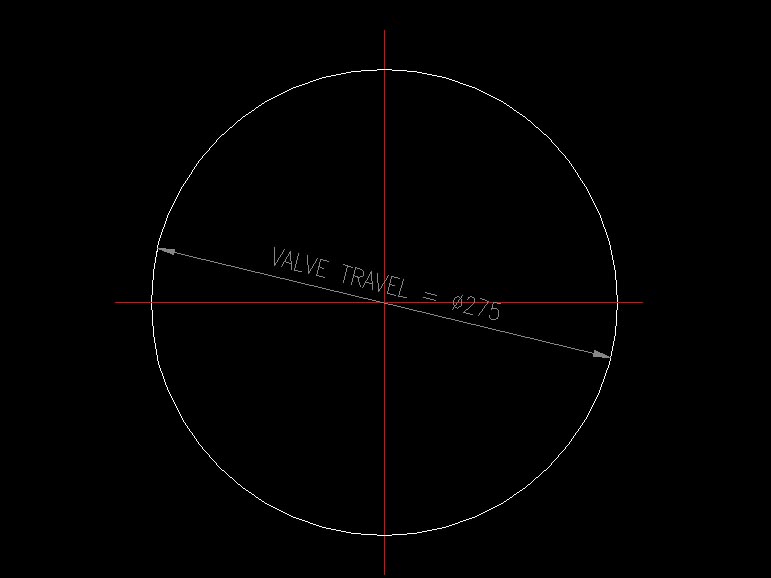
2) Now draw two lines parallel to the vertical axis, one offset by the steam lap, and the other by the lead – in this case 65mm and 7mm respectively:
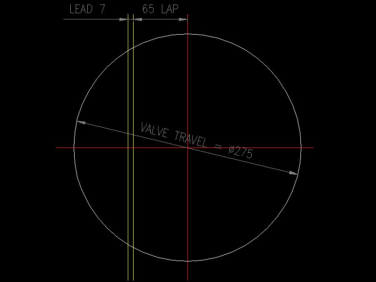
3) Draw a diameter from the point where the Lead line intersects the circle, and another diameter at right-angles to it.
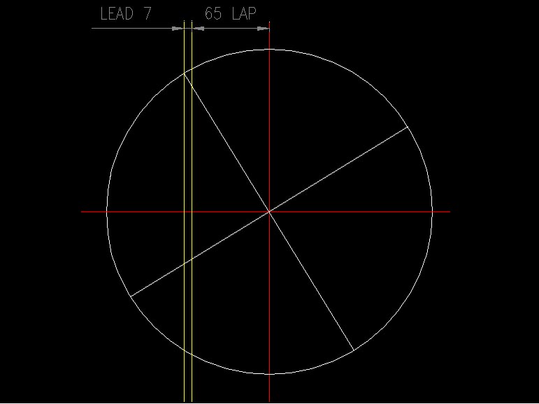
4) Draw two lines parellel to the last-drawn diameter, the first offset on one side by the steam lap (65mm) and the second offset to the other side by the exhaust lap (18mm).
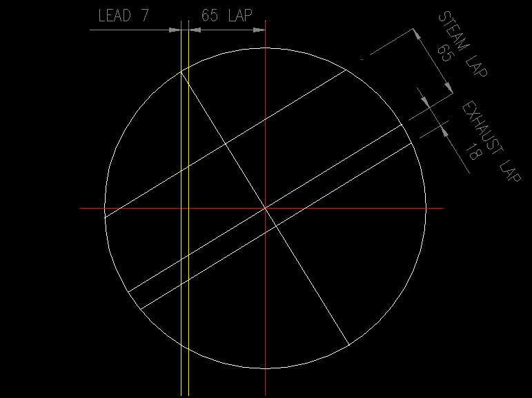
5) It will be discovered that the distance between the upper (steam lap) line and the nearest axis of the circle exactly equals the lead (7mm). Draw Admission, Cut-off, Release and Compression lines as shown below.
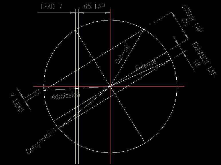
6) Draw verticals from the points where the Admission, Cut-off, Release and Compression lines meet the circle. The distances from the edge of the circle represent the point where each valve event occurs. These distances can be converted to percentages – see below.
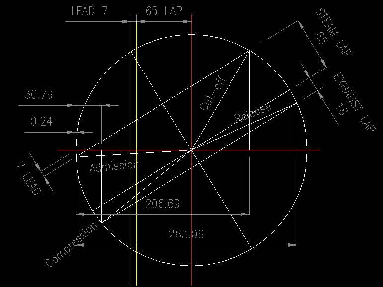
From the diagram above:
- Cut-off occurs at a distance of 206.69mm from the left of circle. 206.69 ÷ 275 = 0.7516 = 75% (i.e. maximum cut-off);
- Release occurs at 263.06 mm or 263.06 ÷ 275 = 0.9566 = 96%
- Compression occurs at 30.79 mm = 30.79 ÷ 275 = 0.1119 = 12%
- Admission occurs at 0.24 mm = 0.24 ÷ 275 = 0.0009 = 0.1%
Simple and Compound Expansion
The term “Simple Expansion” refers to the single use of steam in powering a steam engine. “Compound Expansion” refers to the multiple uses of steam in powering a steam engine.
In a “simple” engine, the steam enters the cylinder at high pressure, expands as it pushes the piston through its stroke, and is then exhausted to atmosphere as the piston returns, whereas in a “compound” engine, the exhausted steam is reused in a second “low pressure” cylinder where it expands further as it pushes the low pressure piston through its stroke. In the case of a double expansion compound, the steam will then exhausted to atmosphere. In a triple-expansion compound (mostly used in marine applications) the steam is reused again in a third (even lower pressure) cylinder.
In a compound engine, the steam will pass from the high pressure cylinder into a “receiver” (a pipe or pressure vessel of adequate volume) before being admitted into the low pressure cylinder. In some cases, the receiver will incorporate means of re-superheating the steam to raise its temperature to minimize the risk of condensation.
In historical texts, proponents of compound expansion are reputed to have claimed that greater use is made of the steam by expanding it twice (or more) thereby increasing the work it does and the efficiency achieved, whereas proponent of simple expansion are reputed to have claimed that the simplicity and lower cost of simple engines outweight the efficiency gains offered by compound expansion.
In fact the arguments for and against compound expansion are more complex – and too complex to expound on a website such as this and are more adequately covered elsewhere – for instance
- http://hubpages.com/hub/10-Advantages-of-Compound-Steam-Engine lists ten (easy-to-understand) advantages of compound expansion.
- Col. Roger’s biography of Chapelon also offers an excellent (and not overly technical) background on the subject; and
- Porta’s “Fundamentals of the Porta Compound System for Steam Locomotives” gives greater technical insight as explained further in the Compound Expansion page of this website.
However a few simple and pertinent points are worth summarizing here:
- Use of compound expansion allows longer cut-offs to be used, thereby delivering more uniform wheel-rim tractive effort;
- The ability of compound engines to operate efficiently at longer cut-offs increases their α-coefficient and thus their power-to-weight ratio.
- The reduction in vibration (or knocking) achieved from the use of longer cut-offs removes the incentive to operate a locomotive with a throttled (partially opened) regulator, thereby allowing full boiler pressure in the steamchest;
- More uniform torque delivered by compound locomotives reduces the propensity for initiation of wheel-slip at moments of (transient) peak torque. This renders compound locomotives better suited to heavy haulage;
- Reduced temperature differentials between steam entering and leaving a cylinder, minimizes heat losses and reduces or eliminates condensation, especially where the low-pressure steam is re-superheated.
Notwithstanding the above, Wardale has adopted simple expansion for the 5AT for several reasons. most of which are outlined in an FAQ on the subject:
- Wardale has no personal experience of compound locomotives to draw on or upon which to base an “assured” locomotive design;
- Wardale believes that for a high-speed locomotive such as the 5AT simple expansion – using all the cylinder refinements that are now possible, but which are not common knowledge – is the right choice, and that the 5AT will define ‘state of the art’ for 2-cylinder simple locomotives and may serve as a reference level to which the performance of all other types of locomotive (including compounds) can be compared.
- Such improvement in thermal efficiency that might be gained by compound expansion cannot guarantee to justify the extra design complexity and higher manufacturing costs involved.
- The limited low pressure cylinder volume possible within the British moving structure gauge, with a conventional layout of the cylinders, is an important limiting factor on compound design and performance.”
Steam Chest
The steam chest (or steamchest) is the “reservoir” for collection of steam as it passes between the superheater header and the inlet port to the cylinder.
The advantage of a large steam chest (as is the advantage of any reservoir) is that fluctions in pressure as the steam passes from the steamchest into the cylinder are reduced. The higher the steamchest pressure, the greater the quantity of steam that can be delivered to the cylinder while the inlet port is open, and the higher the cylinder pressure at the point of cut-off. Maximizing cylinder pressure at the point of cut-off serves to maximize the work done by the steam on the piston. In alternative words, it serves to maximize the area within the indicator diagram.
Ideally, the steamchest volume should equal (or exceed) the cylinder volume, but never came near this in FGS locomotives. One of the modifications that Wardale made in developing The Red Devil was enlargement of the steam chests which are easily visible on the photo below. In fact, the extent of the enlargement was limited by other constraints such that their volume increased only from 33.2% of cylinder volume to just 35.5% compared to an ideal minimum of 100%. By contrast, the 5AT steam chest volume is almost exactly 100% – see line [158] of FDC 6.
Cylinder Clearance Volume
The clearance volume of a cylinder (often presented as a percentage term) is that part or proportion of the cylinder volume that is not swept by the piston. It is therefore the volume (or proportion of total volume) taken up by the steam passages and cylinder-head cavities – i.e. the volume contained between the piston head and valve port when the piston is at dead-centre.
![]()
Ideally, the clearance volume should be as small as possible because that part of the steam that fills the clearance volume at the end of each stroke is wasted in that it has done no “work” on the piston. However reducing the clearance volume also necessitates reducing the area of the steam passages which has the effect of restricting steam flow in and out of the cylinder. Furthermore, low clearance volume can result in very high compression that can cause cylinder cover pressure release valves to blow, which is reported to have been a tendency on GW King Class 4-6-0s that clearance volumes of around 6%.
A compromise has therefore to be adopted and the clearance volume of most latter-day steam locomotives has been in the order of 10%. In the case of the 5AT with its double-valve arrangement, Wardale adopted a clearance volume of 10.6%.
In his “Compounding” paper published in Camden’s book “Advanced Steam Locomotive Development – Three Technical Papers“, Porta makes the following observations relating to Clearance Volume:
“Fig. 19 (below) shows the influence of the clearance volume: for high boiler pressures it requires prohibitive compressions (thus spoiling the (alpha coefficient) much as happens in compressors. The convenience of a small clearance volume was appreciated early on by Churchward, but his preaching was not understood: he came down to 6% – current engines show 12% and even more in the case of poppet valves.

The ideal engine, with zero clearance volume, working at 11% cut-off, operates along the cycle 1-2-3-4-5-1 and shows the area A as the incomplete expansion loss. Should 11% clearance volume be included, the cycle becomes 2′-3′-4′-5′-2′, and the incomplete expansion loss (area B) becomes much greater.”
A separate page of this website is dedicated to the subject of incomplete expansion losses.
Note: in the case of compound expansion engines, Porta recommends that a relatively large clearance volume be provided in the high-pressure cylinder(s) in order to avoid over-expansion at short cut-off working. He suggests a figure of around 16%, but notes that in the case of his 3-cylinder scheme, he adopts a figure of 35%. In the case of the low pressure cylinder(s) however, clearance volume should be as small as possible, as with single/simple expansion engines.
Several pages of this website include text and diagrams copied from Porta’s “compounding” paper, including the pages covering condensation/wall effects, steam leakage, incomplete expansion and triangular losses. More specific references to his theories on compound expansion can be found on the α Coefficient and Compound Expansion pages.
Sincere thanks to Adam Harris of Camden Miniature Steam, publishers of “Advanced Steam Locomotive Development – Three Technical Papers” for allowing the sections of the book to be published on this website.
Snifting, Drifting, Bypass and Herdner Valves
Snifting, Bypass and Drifting Valves were commonly used as a means of preventing negative pressures occurring in the cylinders of a locomotive during “drifting” or free-wheeling. If a negative pressure does occur, it will immediately result in combustion gases and solid particulates being sucked down from the smokebox through the blast pipe, causing serious abrasion damage to the rubbing surfaces of both pistons and valves.
- Snifting valves are simple one-way “check-valves” that allow clean air to be sucked into the cylinder in the event of negative pressure arising. These were commonly mounted on the side of the locomotive’s smokebox from where clean air could be drawn, thereby causing (undesirable) cooling of the cylinders. Furthermore, admitting air into the steamchests and cylinders can result in oxydation of lubricants and the formation of deleterious gums, as described on the Tribology page of this website. Snifting valves can also leak, with obvious detremental effects. For further information see http://en.wikipedia.org/wiki/Snifting_valve.
- By-pass valves simply allow steam (or air) to pass from one end of the cylinder with the other through a linking duct or chamber. They are automatically closed by the admission of live steam to the steam chest and opened when the steam supply is shut off. The main problem with use of these valves was steam leakage. For diagram, see http://www.nwhs.org/qna/BypassValves.html.
- Drifting valves differ from Snifting and By-pass valves, in that they admit a small quantity of live steam into the cylinder during drifting in order to prevent the creation of a vacuum in the cylinder. Drifting valves are often incorporated into the design of the regulator.
Some railways (for instance the South African Railways) incorporated all three of these anti-vacuum valves into their locomotives, and encouraged their drivers (“engineers” in the US) to set their machines to drift in full forward gear, thereby relying on these devices to prevent any admission of gases from the smokebox.
In modifying SAR 2644 and 3450 “The Red Devil” Wardale stripped all three devices off both locomotives.
Wardale took sample indicator diagrams when running using three methods of drifting:
- valves in mid-gear; throttle shut;
- valves in full-gear; throttle cracked open.
- valves in mid-gear; throttle cracked open.
In case 1, he detected a momentary vacuum in the cylinder; in case 2, the steam flow became far too high; case 3 was found to be satisfactory, and was therefore recommended as the operating regume to be adopted for both locomotives.
See also Drifting Techniques page.
Herdner Valves are simple non-return valves that are fitted to the mid-points of a locomotive’s cylinders. When opened, they admit steam directly from the steamchest into the cylinder, the steam flow being continuous regardless of the piston valve position. As the piston moves from the end to the mid-point of the cylinder, steam admitted through the Herdner valve escapes directly to exhaust. As the piston moves past the centre position, steam from the Herdner valve applies pressure to the piston until the valve reaches the point of release when the steam once again escapes to exhaust.
Steam is therefore wasted while the locomotive starts its train, but the starting cut-off is effectively increased to around 90% (as measured by the position of the piston at the point of release). Once the train is started, the Herdner valve can be closed and steam flow to the cylinders is controlled normally – i.e. by the piston valves.
The photos below, taken from Wardale’s book “The Red Devil and Other Tales from the Age of Steam” show a Herdner starting valve mounted on the side of the cylinder of The Red Devil itself.


Dynamic Augment or Hammer Blow
Hammer Blow or “Dynamic Augment” is a dynamic force imposed through the driving wheels and onto the railway track resulting from the rotation of out-of-balance weights that are attached to the driving wheels for the purpose of counteracting the horizontal inertia forces resulting from the “to-and-fro” motion of the reciprocating motion parts.
Balancing of locomotives is a highly technical subject that is not (as yet) discussed in detail here. However a quick understanding of the principles of balancing and hammer blow could be derived from http://home.new.rr.com/trumpetb/loco/ but since the site is no longer accessible, the text and diagram from it are reproduced below:
Why Are the Main Driver Counterbalances Not Symmetrical?First, recall that locomotive drivers are quartered; ie: the right/left connecting rod pins are oriented 90 degrees apart. As one crank is on dead center, the other is at the position of maximum torque, and the power strokes are evenly spaced throughout the driver rotation. It appears that most locomotive drivers are quartered with the right side leading by 90 degrees, as illustrated. (At least one example however, PRR K-4s #1361, has ‘left hand lead’.)
What may not be obvious is that the counterbalances are doing more than simply statically balancing the crank pin, side rods, main rod, and eccentric crank on their respective sides. The main driver counterbalances are “tipped” to provide a force component on one side (eg: left) to cross-balance a rocking couple caused by the opposite (eg: right) side rods and eccentric crank about their own counterbalance weight. This cross balancing renders the axle/driver assembly in dynamic balance as well as static balance. This concept is applicable for all axles, but apparently was done only for the main axle where the additional mass and larger moment arm of the main rod and eccentric crank is much more significant. Additionally, notice that the eccentric crank tips a different direction on each side of the locomotive (when the side rod is down the eccentric crank slants toward the front of the locomotive for normal inside admission valve gear). The main axle counterbalance position takes this into consideration also, contributing further to irregularity of the counterbalance weights. [A site visitor commented that few if any American locomotives were cross-balanced before around 1930. Our example Soo #2714 Pacific may have gotten the cross-balanced counterweight design with the Boxlike main driver conversion (ca. 1951?). However, another visitor (thanks, John) cites Union Pacific/AlCo 4-12-2s, designed during 1925, as having noticeable evidence of cross-balancing on both main driving axles (“tipping” of the counterbalance lunes).] In the context of balance, it should be mentioned also that for this type of two cylinder (single cylinder per side) locomotive, the counterbalance weights balance all of the rotating mass per the above, but balance only a portion of the reciprocating mass. The rotating mass (crank pins, each end of the side rods, back portion of main rod) can be theoretically perfectly balanced with counterbalance weight. However, the reciprocating mass (piston assembly, piston rod, crosshead, union link, bottom portion of combination lever, front part of main rod) cannot be balanced with the driver counterbalances. Any attempt to balance reciprocating mass only results in trading off horizontal unbalance for a vertical unbalance component (overbalance). This overbalance force, referred to as hammer blow, increases with the square of the velocity and is an undesirable characteristic of steam locomotives that was damaging to railbeds and bridges at higher speeds. |

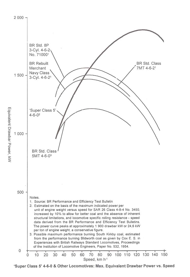
Further information on the subject of Balancing and Hammer-blow can be found from many sources including the following:
- Wardale, D.W., Fundamental Design Calculations for the 5AT – FDC 8 “Balancing” (unpublished) from which some notes on FDC 8 are published on this website.
- Jarvis, J.M., Balancing of the BR Class 9 2-10-0 Locomotives (transcribed from an SLS journal) – a fascinating account of how the balancing of these remarkable locomotives was worked out with some explanation of balancing techniques and alternative approaches to balancing.
- Wikipedia’s article on the subject.
Locomotive and Train Brakes
There are three types of brakes used in railway operations: the Air Brake, the Steam Brake and the Vacuum Brake.
Steam Brake (steam locomotives only): steam brakes are used only on steam locomotives and their tenders. Steam brakes use the steam from the locomotive’s boiler to generate the braking force that are applied to the wheels of the locomotive and tender.
Automatic Vacuum Brake (heritage trains only): developed in the UK in the second half of the 19th century, the automatic vacuum brake was widely used in the UK and in other countries that adopted British technology, until air brakes became the standard in the late 20th century. Vacuum braking is still used on heritage railways in the UK and on some main line railway systems in Africa and India.
Dominic Wells has produced an excellent PowerPoint presentation that describes in great detail the operation of the train brakes. The first part (pages 1 to 205) focuses on Vacuum Brake operation.
Air Brakes: the most widely used brake system is the air brake which uses compressed air to generate the necessary force to apply the brakes throughout the length of a train. Air brakes are universally used on modern railway rolling stock worldwide. The second part of Dominic Well’s presentation (pages 206 to 324) describes Air Brake operation.
Thermodynamics
Draft Text Only – Readers’ suggestions and inputs are welcome
Introduction
Oliver Bullied, disciple of Gresley and famously progressive CME of the Southern Railway, is often quoted as saying “Thermodynamics never sold a single locomotive” (or words to that effect) when commenting on Chapelon’s contemporary locomotive developments in France. Whether true or apocryphal, the remark exemplifies the lack of understanding of Thermodynamics that was widely prevalent within the locomotive engineering fraternity of his day. Indeed it remains poorly understood by many engineers today, and is a complete mystery to most laymen.
In fact, the study of Thermodynamics is still evolving to the extent that it now spreads far beyond the mysteries of steam power that inspired its early development. The author of the web page http://thermodynamicstudy.net/history.html offers a broad view of its modern day scope:
The history of thermodynamics [is] not only one of the most interesting but one of the most dramatic episodes to be found in the story of the intellectual progress of the human mind. Starting in an investigation of a purely practical problem of engineering economics, it has grown into a body of doctrine of profound philosophical significance, with consequences which permeate the thinking of men on many subjects, from those with the most practical use to the problems of cosmology.
This page and the sub-pages under it, attempt to explain the rather esoteric and abstract concepts that underlie the subject of thermodynamics as it applies to steam traction, using terms that it is hoped will be more readily understood than those found in most texts on the subject.
History of Thermodynamics:
Many scientists of past ages could claim to be the “father of Thermodynamics” but it is probably most useful to give the credit to Nicolas Léonard Sadi Carnot, a young French military engineer who in 1824 set out to determine how the greatest amount of mechanical work could be obtained from a given amount of heat. In so doing, he invented the idea of the Carnot Cycle, being an idealized concept from which the maximum theoretical efficiency of any heat engine can be determined through the simple equation:
Carnot efficiency = (1 – T2/T1) where T1 and T2 are the temperatures
of the heat source and heat sink respectively, measured in oK.
It was not until the 1920s that André Chapelon began to apply the theories of Thermodynamics to the design of steam locomotives, with immediate and dramatic results. Unfortunately his work remained poorly understood in most steam locomotive design offices around the world and it was only in the 1950s that Livio Dante Porta took up the mantle and continued the work that Chapelon had started.
Important amongst the many lessons that Chapelon (and Porta) learned from Thermodynamics comes from Carnot’s simple equation which explains the importance of high temperature superheat since it shows that an engine’s efficiency is critically affected by its temperature. In the case of a typical “first generation” steam locomotive operating at a superheat temperature of (say) 350oC and with an exhaust steam temperature of (say) 180oC, its theortetical (maximum) Carnot efficiency would be 27%, whereas the 5AT operating at a superheat temperature of 450oC and exhausting at 183oC, its theortetical (maximum) Carnot efficiency is 37%.
[Note: Carnot’s theorem derives efficiency values that are purely theoretical. His equation does not apply specifically to steam engines but to all types of heat engine – steam, diesel, Stirling or any other. The purpose of comparing Thermodynamics dictates through Carnot’s Theorem that any heat engine’s efficiency is limited by the temperature differences between which it operates. See also Superheating page]
Laws of Thermodynamics
The study of thermodynamics is defined by three relatively simple laws:
-
First Law – energy can be neither created nor destroyed, or “energy is conserved”;
-
Second Law – energy will tend to dissipate from a hot or high energy body to a cold or low energy sink – or “heat cannot spontaneously flow from a cold body to a hot one”;
-
Third Law – defines absolute zero as equalling -273oC, being the hypothetical point at which energy becomes zero.
In fact the Second Law can be written in many different ways. Here is another one:
-
Alternative Second Law: It is impossible to extract an amount of heat from a hot source and use it all to do work. Some amount of heat must be exhausted to a cold sink. This precludes a “perfect” heat engine.
Whilst the laws themselves are simple enough, the interpretation of them leads to complications. Most notably, the Second Law involves understanding the concept of Entropy. The concepts of Entropy and Enthalpy are described in separate sub-pages, together with a brief explanation of what “Steam Tables” are about.
There are a wide range of interpretations covering the concepts of Thermodynamics that can be found on several websites including the following:
- http://en.wikipedia.org/wiki/Carnot_heat_engine
- http://fr.wikipedia.org/wiki/Sadi_Carnot_(physicien)
Page Under Development
This page is still “under development”. Please contact the webmaster@advanced-steam.org if you would like to help by contributing text to this or any other page.
Definitions of thermodynamic concepts such as Entropy and Enthalpy are provided on separate pages of this website. Numerous useful (and often diverse) definitions of these and other terms can be found on the Internet.
A particularly useful (and brief) discussion can be found here (from http://www.mathpages.com/home/kmath184/kmath184.htm).
Adiabatic Process
An adiabatic process is one in which there is no transfer of heat between the system and its surroundings. Thus in thermodynamic nomenclature, Q (heat transfer to or from a system) = 0
Adiabatic expansion can occur in a well-insulated system. Neglecting kinetic energy, electrical energy, etc, the drop in enthalpy of the system is effectively converted to work (dH = Q + W, where Q = 0). An adiabatic expanion is thus considered to be most expanion that can occur.
Adiabatic Efficiency is the ratio of the actual work output of the engine to the work output that would be achieved if the process between the inlet state and the exit state was isentropic (see below).
Isentropic (or Isoentropic) Process and Isentropic Efficiency
An isentropic process is an ideal or “perfect” process in which entropy remains constant. For a reversible isentropic process, there is no transfer of heat energy and therefore the process is also adiabatic.
If a process is both adiabatic and reversible, then it is considered to be isoentropic.
Isentropic expansion of steam is represented as a vertical line on a Mollier h-s diagram. However expansion of steam is never perfect and some increase in entropy cannot be avoided. Real expansion is represented by a sloping (non-vertical) line, the angle of slope being indicative of the isentropic efficiency of the expansion.
In the case of a steam locomotive, the isentropic efficiency of the expansion of steam in the cylinder is found by dividing the specific work done in the cylinder by the isentropic heat drop between admission and exhaust. It therefore defines the efficiency of the engine unit (i.e. cylinders, valves etc) in terms of the amount of work it delivers from each stroke compared to the isentropic heat drop of the steam between admission and release.
Isentropic efficiency is therefore a measure of the efficiency of the engine unit. As with a locomotive’s thermal efficiency, its isentropioc efficiency varies with speed, cut-off, steamchest pressure etc.
An example appears in the 5AT FDCs, where lines 68 to 84 of FDC 1.3 are used to calculate the isentropic efficiency of the 5AT at maximum drawbar power.
An example of isentropic efficiency being applied in a calculation can be found here.
Isenthalpic (or Isoenthalpic) Process
An isenthalpic process is one that proceeds without any change in enthalpy (H) or specific enthalpy (h). There will usually be significant changes in pressure and temperature during the process.
In a steady-state, steady-flow process, significant changes in pressure and temperature can occur to a fluid. However the process will be isenthalpic if
- there is no transfer of heat to or from the surroundings (i.e. it is adiabatic),
- there is no work done on or by the surroundings, and
- there is no change in the kinetic energy of the fluid.
The throttling process is an example of an isenthalpic process – for instance the lifting of a safety valve on a steam boiler. The specific enthalpy of the steam inside the boiler is the same as the specific enthalpy of the steam as it escapes from the valve. Thus with a knowledge of the specific enthalpy of the steam and the pressure outside the pressure vessel, it is possible to determine the temperature and speed of the escaping fluid.
In an isenthalpic process: h1 = h2 and therefore dh = 0.
The above definition comes from Wikipedia and also World Lingo which offers an almost identical definition. However neither is entirely satisfactory since steam escaping through a safety valve will experience rapid cooling in its surroundings. The diagram below (from Chemical and Process Technology) gives a clearer picture even if the accompanying explanation is less so.
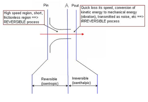 An interpretation of the accompanying explanation is offered as follows:
The flow through a pressure relief valve is extremely fast. Choked flow can occurs as far as position A inside the nozzle. The flow from the inlet to “A” will be a REVERSIBLE process and thus an ISENTROPIC process. Beyond “A” to the outlet of the valve, the steam expands (it may even undergo a change in state if it is liquid prior to “A” resulting in a transformation energy loss) followed by a rapid loss of speed and conversion of kinetic energy to mechanical energy in the form of noise. However the enthalpy remains constant (ISENTHALPIC). This process is IRREVERSIBLE (i.e. entropy increases).
Heat Capacity Ratio, Isentropic Expansion Factor, or Expansion Coefficient
[Ref Wikipedia] The Heat Capacity Ratio is sometimes also known as the “isentropic expansion factor“. In the 5AT FDCs, the expansion factor is termed the “expansion coefficient” and denominated by the letter ‘n’. In other texts it may be denoted by γ, κ or the letter k.
The value of n is derived from the equation: n = Cp / Cv where, C is the heat capacity of a gas, suffix P and V refer to constant pressure and constant volume conditions respectively.
The heat capacity ratio (expansion coefficient) ‘n’ can be visualized from the following experiment:
A closed cylinder with a locked piston contains air. The pressure inside is equal to the outside air pressure. This cylinder is heated to a certain target temperature. Since the piston cannot move, the volume is constant, while temperature and pressure rise. When the target temperature is reached, the heating is stopped. The piston is now freed and moves outwards, expanding without exchange of heat (adiabatic expansion). Doing this work cools the air inside the cylinder to below the target temperature. To return to the target temperature (still with a free piston), the air must be heated. This extra heat amounts to about 40% more than the previous amount added.
In this example, the amount of heat added with a locked piston is proportional to CV, whereas the total amount of heat added is proportional to CP. Therefore, the heat capacity ratio in this example is 1.4.
From Steam Tables the following outputs can be found (based on a pressure of 20 bar)
| Pressure = 20 bar | 200oC | 300oC | 400oC | 450oC | |
| Cv | kJ/(kg.oC) | 2.06657 | 1.696 | 1.66439 | 1.67895 |
| Cp | kJ/(kg.oC) | 2.98955 | 2.32035 | 2.2013 | 2.19664 |
| n | – | 1.35 | 1.37 | 1.32 | 1.31 |
The coefficient is usually given the value 1.3 in SGS locomotive performance calculations.
Reversible Process
A reversible process is a process that, after it has taken place, can be reversed and causes no change in either the system in which the process takes place, and causes no change in its surroundings. In thermodynamic terms, a process “taking place” would refer to its transition from its initial state to its final state. Or put another way, a reversible process changes the state of a system in such a way that the net change in the combined entropy of the system and its surroundings is zero.
Since all processes involve some increase in entropy (however small), the concept of reversibility is an ideal one that can never be achieved in practice. However the concept of reversible processes is a useful one. For instance, it is used to define the maximum possible efficiency (the isentropic efficiency) of a heat engine in that a reversible process is one where no heat is lost from the system as “waste”, and the machine is thus as efficient as it can possibly be (see Carnot cycle).
A reversible process is thus of necessity an isentropic process.
Specific Volume: Specific volume of a gas is the inverse of its density. It is therefore a measure of volume per unit of mass. In steam tables, its units are usually given as m3/kg (or lb/ft3 in the old units).
Page Under Development
This page is still “under development”. Please contact the webmaster@advanced-steam.org if you would like to help by contributing text to this or any other page.
Thermodynamics Nomenclature:
| T = temperature (oK) |
| V = volume of system (cubic metres) |
| P or p = pressure at the boundary of the system and its environment, (in pascals) |
| W = work done by or on a system (joules) |
| Q = heat transfer in or out of a system (joules) |
| q = specific heat transfer in or out of a system (joules per kg) |
| U = internal energy of a system mainly contained in solid and liquid components (joules) |
| u = specific internal energy of a system (joules per kg) |
| H = enthalpy of a system (joules) |
| h = specific enthalpy (joules per kg) |
| S = entropy (joules per oK) |
| s = specific entropy (joules per kg per oK) |
| n = heat capacity ratio (= Cv/Cp) |
Thermodynamics Equations:
Thermodynamics equations can be difficult to understand. The following is a simpified summary where the term “system” can be equated to a steam locomotive’s cylinder:
The First Law of Thermodynamics (conservation of energy) can be expressed as “The increase in internal energy of a system = the heat supplied to the system minus the energy that flows out in the form of Work that the system performs on it environment” [ref Wikipedia]. In this case, the external “environment” is the locomotive’s piston, hence the definition can be formulated by the equation:
δU = Q – Wpiston ………… (1)
which may also be written:
dU = dQ – dWpiston ………. (1a)
However, the work done on a system (locomotive cylinder) by changing its volume is dW = p.dV, hence:
dU = dQ – p.dV …………. (1b)
If the process (steam expansion) is assumed to be adiabatic – i.e. with no heat transfer in or out, then dQ = 0, whence
dU = – p.dV ………………. (1c)
However Enthalpy is defined as the sum of a system’s internal energy plus the product of its pressure and volume – i.e.
H = U + P.V ……………..(2)
from which a change in enthalpy can be defined (by differentiation) as
dH = dU + p.dV + V.dp ……………..(2a)
Thus by combining equations (1c) and (2a) we get (for adiabatic expansion): dH = -p.dV + p.dV + V.dp, or
dH = V.dp ……………..(3)
Combining eqns (1c) and (3) gives:
dH/dU = – V.dP / P.dV …………….. (4)
The Second Law of Thermodynamics (heat always flows to regions of lower temperature) can be expressed as “a change in the entropy (S) of a system is the infinitesimal transfer of heat (Q) to a closed system driving a reversible process, divided by the equilibrium temperature (T) of the system” [ref Wikipedia]. This definition is formulated by the equation:
dS = δQ/T or dQ = T.dS ………………(5)
By combining Eqn (4) with (1b), a change in internal energy is given by:
dU = T.dS – p.dV ………………………….(6)
Ideal Gas Laws (from physics): The ideal gas law is defined by the equation:
pVn = k …………………………. (7)
where n is the “heat capacity ratio“: n = Cp / Cv = – V.dp / p.dV [ref Wikipedia]
Thus from equation (4):
n = dH/dU
———— page in progress as at 10th Mar 2011 ———–
Enthalpy is a “term of convenience” that is useful in the interpretation and application of Thermodynamics. Enthalpy is basically a measure of energy, but its main function is in the calculation and measurement of “flow energy” or gaseous energy (e.g. steam energy).
[Note (borrowed from mathpages.com): Enthalpy is not a specific form of energy. It is just a defined variable that often simplifies calculations in the solution of practical thermodynamic problems.]
The term enthalpy is defined as the sum of a system’s internal energy plus the product of its pressure and volume, or
H = U + P x V
-
where H is the enthalpy of the gas (in Joules),
-
U is its internal energy (in Joules),
-
P is its pressure in Pascals, and
-
V is its volume in cubic metres.
Put another way, Enthalpy = Internal Energy + Flow Energy.
Commonly a “system” may be a combination of solids, liquids and gases, in which case most of its internal energy applies to the solid and/or liquid components while the PV term defines the energy of the gaseous component. This is confirmed by looking at steam tables which show that the enthalpy of water (in its liquid phase) is almost identical to its internal energy.
Specific enthalpy (usually denoted by the lower-case letter ‘h’) is the enthalpy per unit of mass, often measured in units of kJ/kg.
Measurement or calculation of a change in enthalpy is usually more meaningful than the value itself. For instance, the energy inputs required to raise and superheat steam can be estimated from the change in enthalpy between each step of the process. The first table assumes that cold feedwater is injected into the boiler before being heated; the second table assumes that the feedwater is preheated to 100oC before entering the boiler (in both cases taken to be at a pressure of 20 bar = 2000 kPa):
| Enthalpy Rise without Feedwater Heating |
|||
| 1 Start with cold water | Enthalpy of water at 25oC | 105 kJ/kg | Increase |
| 2 Raise water pressure to 20 bar | Enthalpy of water at 20 bar and 25oC | 107 kJ/kg | 2 kJ/kg |
| 3 Raise water temperature to 212oC | Enthalpy of water at 20 bar and 212oC | 909 kJ/kg | 802 kJ/kg |
| 4 Evaporate at same temp & pressure | Enthalpy of steam at 20 bar and 212oC | 2798 kJ/kg | 1890 kJ/kg |
| 5 Superheat steam to 400oC | Enthalpy of steam at 20 bar and 400oC | 3248 kJ/kg | 450 kJ/kg |
| 6 Total of enthalpy rises from point 1 to point 5 = 3248 – 105 = | 3143 kJ/kg | ||
| Enthalpy Rise with Feedwater Heating |
|||
| 1 Start with cold water | Enthalpy of water at 25oC and 1 bar | 105 kJ/kg | Increase |
| 2 Raise water pressure to 20 bar | Enthalpy of water at 25oC and 20 bar | 107 kJ/kg | 2 kJ/kg |
| 3 Raise water temperature to 100oC | Enthalpy of water at 20 bar and 100oC | 418 kJ/kg | 311 kJ/kg |
| 4 Raise pressure to 20 bar | Enthalpy of water at 20 bar and 212oC | 909 kJ/kg | 491 kJ/kg |
| 5 Evaporate at same temp & pressure | Enthalpy of steam at 20 bar and 212oC | 2798 kJ/kg | 1890 kJ/kg |
| 6 Superheat steam to 400oC | Enthalpy of steam at 20 bar and 400oC | 3248 kJ/kg | 450 kJ/kg |
| 7 Total of enthalpy rise from point 1 to point 6 = 3248 – 105 = | 3143 kJ/kg | ||
It can be seen from step 2 of this second table that pre-heating of the feedwater to 100oC reduces the energy required from the firebox by around 10%, hence offering a potential nominal fuel saving of this amount. [Note: if preheat is obtained from exhaust steam, then the resulting loss of energy from the exhaust will result in a small loss in exhaust system performance and thus a slight increase in cylinder back-pressure and loss of cylinder efficiency. This loss, however, is far outweighed by the overall efficiency gain from feedwater heating.]
It can also be seen from both tables that the additional energy required to superheat the steam is small compared to the amount required to boil the water. The advantage of using superheated steam is that all of the energy in the steam can be put to use in the cylinder provided the degree of superheat is high enough to prevent the occurence (momentary or otherwise) of condensation in the cylinder.
For further information on the subject of enthalpy, see:
Entropy
Draft Text Only – Readers’ suggestions and inputs are welcome
When a car or locomotive runs or brakes, we say that the heat escaping from it is “lost”. The Second Law of Thermodynamics explains this by saying that “energy will tend to dissipate from a hot or high energy body to a cold or low energy sink”. However since the First Law states that “energy cannot be created or destroyed”, then the “lost energy cannot simply disappear.
The concept of entropy was invented to account for this anomaly. This “waste heat” (or waste energy) dissipates into the atmosphere which acts as a heat sink, absorbing the energy without measurable increase in temperature. In so doing, the absorbed heat or energy effectively becomes “useless” (or wasted) to the extent that it cannot be put to further practical use.
Merriam Webster’s on-line dictionary offers three reasonably understandable definitions of entropy as follows:
-
a measure of the unavailable energy in a closed thermodynamic system that is also usually considered to be a measure of the system’s disorder, that is a property of the system’s state, and that varies directly with any reversible change in heat in the system and inversely with the temperature of the system; broadly : the degree of disorder or uncertainty in a system;
-
the degradation of the matter and energy in the universe to an ultimate state of inert uniformity;
-
a process of degradation or running down or a trend to disorder.
A better defintion comes from mathpages.com which offers the following: “The property that we call entropy is a measure of the uniformity of the distribution of energy”. It goes on to state that the entropy of a system equals the sum of the entropies of its component parts.
In simplistic terms, entropy can be thought of as a means of quantifying degraded or “useless” energy. The flame in a locomotive firebox contains a high concentration of energy (enthalpy) and a relatively low entropy, while the (lower temperature) steam in the boiler has a lower enthalpy and greater entropy. Exhaust steam leaving the chimney has an even lower enthalpy and higher entropy.
In fact, contrary to Merriam Webster’s definition, entropy is not a measure of energy. This may be deduced by the fact that by definition, the entropy of a closed system (e.g. the universe) gradually increases over time and is therefore not conserved. Entropy is in fact defined in units of energy per unit of temperature, as per the equation S1 – S2 = δQ/T where δQ represents a (small) amount of heat transfer to or from a body, T is its temperature and S1 and S2 its entropy before and after the energy transfer. The equation can be written dS = dQ/T giving entropy in units of energy per unit of temperature.
Specific entropy is the entropy of a system (usually a gas) divided by its mass, or in other words its entropy per kg in units of Joules per kg per oK.
In practical steam locomotive terms, values of specific entropy are usually found by looking them up in a set of steam tables or deriving them from a steam table program.
For further information see:
There are six interrelated properties that define the state of steam:
- Temperature
- Pressure
- Dryness Fraction (within the saturated zone)
- Enthalpy
- Internal energy
- Entropy
Fixing the value of any two properties defines the value of all the others. Thus fixing the values of Enthalpy and Entropy is sufficient to define Temperature, Pressure and Internal Energy of the steam.
The term “Mollier diagram” (named after Richard Mollier, 1863-1935) refers to any diagram that features Enthalpy on one of the coordinates. Commonly used Mollier diagrams are the enthalpy-entropy (or h-s) diagram (below) and the pressure-enthalpy diagram illustrated at the bottom of this page.
The Enthapy-Entropy or h-s diagram:
The h-s diagram is one in which Enthalpy values form the vertical axis and Entropy the horizontal axis. The values of the other related properties may be superimposed in the form of supplementary curves.
In the diagram below:
- green lines show steam temperature;
- blue lines give (absolute) steam pressure; and
- red lines give the dryness fraction (in the saturated zone).
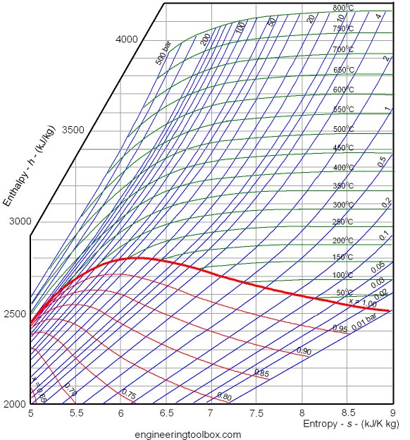
Ideal (isentropic) expansion is represented on the Mollier diagram by a vertical line. Actual expansion of steam always involves some losses represented by an increase in entropy.
In the 5AT FDCs, Wardale gives examples of this, for instance in lines 68 to 84 of FDC 1.3 where he calculates the isentropic efficiency of the 5AT at maximum drawbar power. Here he assumes that the steam enters the cylinders at an absolute pressure of 21.39 bar and temperature of 450oC shown as point A in the diagram below.
He then assumes that the steam will exhaust at an absolute pressure of 1.5 bar. Thus an isentropic expansion line AB can be drawn vertically at a constant entropy of 7.254 kJ/K kg, with point B being defined by pressure = 1.5 bar.
However in FDC 1.3 line 78 Wardale calculates that the actual exhaust steam enthalpy = 2,803 kJ/kg which allows point C to be located on the 1.5 bar pressure line. Thus the actual steam expansion is defined by the line AC.
The slope of the line AC is indicative of the isentropic efficiency of the expansion: the nearer the line is to vertical, the higher isentropic efficiency. Actual isentropic efficiency is determined by dividing the specific work done in the cylinder (FDC 1.3 line 82) by the isentropic heat drop between admission and exhaust (FDC 1.3 line 83).

Porta used similar lines in his Compounding paper but has simplified them by omitting all the irrelevant lines from his diagrams.
The Pressure-Enthalpy diagram below is an alternative representation of the Steam Tables, where the axes are Pressure (Vertical) and Enthalpy (Horizonatl) and with curves representing temperature (T), entropy (s), specific volume (v), and dryness fraction (x).
The dome-shaped curve represents the limits of saturation – within the dome, steam is saturated.
Note: The same points A, B and C from the diagram above are illustrated in red. In this case the line of constant pressure (BC) is straight and the line of constant entropy (AB) is curved.

Steam Tables
Steam tables used to be (and may still be) published in the form of a small booklet listing values of steam temperature, pressure, specific volume (i.e. the volume of 1kg of steam at a given temperature and pressure), specific entropy, specific enthalpy against various input values, separate sets of tables being provided for saturated and superheated steam.
Nowadays it is easier to find values of enthaly and entropy (and many others) using a computer program, of which many are freely available for download from the internet, a good example being:
-
SteamTab™ Companion from http://www.chemicalogic.com/ producing outputs for both saturated and superheated steam in either metric and imperial units.
-
Calcsoft.zip from http://www.winsim.com/steam/steam.htmll, a DOS based program that works only in imperial units. However it offers additional functionality that allows entry of steam inlet and outlet conditions in order to calculate power output, isentropic efficiency and various other values.
Anomalies in Thermodynamics
Draft Text Only – Readers’ suggestions and inputs are welcome
Thermodynamics is not an easy subject to master and there are many instances where it defies intuitive judgement. The following examples are offered by way of enlightenment and perhaps education:
Steam viscosity increases with temperature
Whilst it is intuitive that liquids become less viscous as they get warmer (e.g. oil becomes thinner as it is heated and syrup gets runnier), the opposite is true for steam. The higher the temperature of superheated steam, the higher its viscosity becomes. The following examples are taken from steam tables:
| Steam Pressure bar (psi) |
Steam Temperature |
Steam Viscosity |
| 17.5 (250) | 205 (saturated) | 15.9 |
| 17.5 (250) | 300 | 20.1 |
| 17.5 (250) | 400 | 24.4 |
The fact that the viscosity of a gas increases as temperature increases is due to the increase in the frequency of intermolecular collisions at higher temperatures (reference: http://www.thenakedscientists.com/forum/index.php?topic=23433.0). The rise in viscosity approximately proportional to the square root of temperature
Enthalpy reduces with increasing pressure
A more challenging and less easily explained anomaly is the fact that at constant temperature, the enthalpy and internal energy of steam falls with increase in pressure.
In his book “Hush-Hush: The Story of the LNER 10000“, the author William Brown quotes from an unidenfied report written circa 1930 that seemed to question the wisdom of high pressure steam in such locomotives as Baldwin’s high pressure compound No 60000 and Gresley’s high pressure compound No 10000 of 1929. The report stated that: “if the (steam) pressure is increased while the temperature remains constant, the superheat and heat content per pound of steam fall off as the pressure is increased. If steam of 200 psi and of 350 psi is expanded from the same temperature under such conditions that the exhaust steam escapes at the same pressure and temperature and with the same heat content in both cases, it follows that the heat taken from the steam in the cylinders and converted into mechanical work will be slightly less with the high than with the low pressure steam. That is, with the same heat content in the exhaust steam, the higher pressure will not give greater thermal efficiency.”
The following examples taken from steam tables illustrate the point:
| Steam Temperature deg C |
Steam Pressure |
Internal Energy |
Enthalpy kJ/kg |
| 300 | 13.8 (200) | 2786 | 3041 |
| 300 | 24.1 (350) | 2764 | 3012 |
Wardale’s explanation of this phenomenon is instructive (quoted below):
The premise is that steam expanded from high pressure will produce less work than that expanded from a lower pressure and the same temperature if both exhaust at the same pressure and temperature. This would be true, but if comparing like-for-like, which is essential for the given conclusion to be made, the mistake arises because they will not exhaust at the same temperature, and the exhaust steam will therefore not have the same heat content in both cases. This is demonstrated in the following table, taking your own figures for temperature and pressure. (Note two things: steam properties are always given for absolute pressure, not gauge pressure, essentially because steam can (and should, wherever possible, i.e. power station turbines) be expanded to below atmospheric pressure (but don’t even think of it for a locomotive, please), and it is enthalpy we must use as the measure of steam thermal energy, not internal energy because as soon as a piston moves flow work is involved (consult a thermodynamics text book).)
From the enthalpy – entropy chart (Porta’s ‘Mollier diagram’) we have as follows:
| Inlet Pressure, psi gauge |
200 |
300 |
| Inlet pressure, bar abs. | 14.81 | 25.15 |
| Inlet temperature, °C | 400 | 400 |
| Inlet steam enthalpy, kJ/kg | 3256 | 3239 |
| Inlet steam entropy, kJ/kg.°C | 7.277 | 7.014 |
| Exhaust pressure, psi gauge | 10 | 10 |
| Exhaust pressure, bar abs. | 1.7 | 1.7 |
| For an isentropic = constant entropy or ideal expansion in both cases: | ||
| Exhaust steam entropy,kJ/kg.°C | 7.277 | 7.014 |
| Exhaust steam enthalpy, kJ/kg | 2731 | 2633 |
| Heat drop = work done, kJ/kg | (3256 – 2731) = 525 | (3239 -2633)= 606 |
| Increase in work done for expansion from higher pressure: |
((606 – 525) ÷ 525) x 100% = 15.4% | |
If the same isentropic efficiency (say 85%) is applied to both cases to give a practical expansion allowing for incomplete expansion loss, etc., the relative values always stay the same.
This gives the correct situation and shows the book’s premise to be wrong because it is based on the false assumption of identical exhaust steam condition for both expansions. However the actual conditions are subject to various factors, making a generalized statement rather meaningless, amongst them:
-
- The above isentropic expansion from 200 psi gauge to 10 psi gauge gives an exhaust steam temperature of about 131°C, which is still superheated. However the corresponding expansion from 350 psi gauge gives saturated steam at 116°C and dryness fraction 0.972, hence condensation losses at the end of this expansion would be high. But the entropy rise associated with imperfect expansion acts to increase the exhaust steam temperature for all expansions and hence reduce any tendency for condensation.
- It is unrealistic to have both expansions start from the same temperature. As the saturation temperature of steam at 350 psi gauge is about 30°C higher than that at 200 psi gauge, if both were superheated to the same temperature the degree of superheat (i.e. the amount by which the superheat temperature is in excess of the saturated temperature) would be that much lower for the former. Rather, as steam at higher pressure would enter the superheater at higher temperature, so the inlet steam temperature at the cylinders would be somewhat higher. This would decrease the tendency for condensation at the end of the expansion.
- Simply comparing ultra-high with normal inlet pressure without specifying the nature of the engine (i.e. simple or compound) is misleading, compound being more suited to the former, simple to the latter. In the case of a compound, the superheat temperature must be set higher as the greater expansion possible in a compound (giving a higher isentropic efficiency, a fundamental reason for compounding) would otherwise result in saturated exhaust steam.